
零、写在前面
lecture04主要围绕两个主题:
-
Attention alternatives:注意力机制的替代方案
- 为什么标准 attention 在长上下文下很贵?
- Linear Attention、Mamba-2、Gated Delta Net、Sparse Attention 等思路如何降低成本?
- 为什么很多新模型采用 attention + alternative module 的混合架构?
-
Mixture of Experts,MoE:专家混合模型
- MoE 是什么?
- 为什么它越来越流行?
- 路由 routing 怎么做?
- 训练 MoE 有什么困难?
- DeepSeek MoE v1/v2/v3 等模型做了哪些设计?
一、Attention alternatives
1.1 为什么需要 Attention alternatives
标准 attention 是:
$$ Attn(Q, K, V) = \rho (QK^T)V $$其中:
ρ通常是 softmax;QK^T的形状是n × n;- 所以计算和存储复杂度与
n²有关。
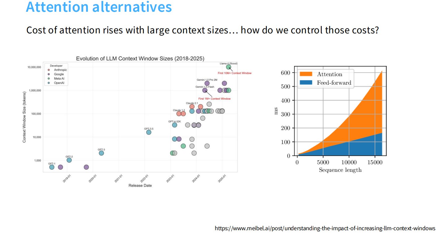
这在短上下文时还可以接受,但当上下文长度变成:32k、128k、1M tokens时,attention 成本会急剧上升。
所以:当 context size 变大时,我们如何控制 attention 的成本?
1.2 控制长上下文成本的基础工具
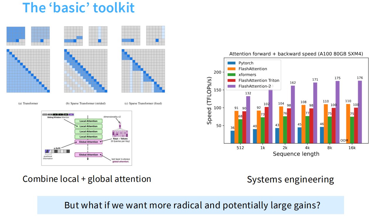
1.2.1 Combine local + global attention
也就是混合局部注意力和全局注意力。
例如:
大多数层用局部窗口 attention
少数层用 full attention
Swin Transformer精读中就引入了局部注意力 与 shifted window 注意力
而且 shifted window 比起 lecture03 提到的sliding window 更加具有访存友好。
1.2.2 Systems engineering
系统工程优化也很重要。
例如:
- FlashAttention;
- KV cache 优化;
- GQA / MQA;
- kernel fusion;
- memory-efficient attention;
- 分布式并行策略。
这些方法不改变 attention 的数学本质,但能显著优化实际运行速度。
1.2.3 更激进的替代方案
讲义接下来关注更激进的方案:
- Linear Attention
- Mamba-2
- Gated Delta Net
- Sparse Attention
- MoE
这些方法希望不仅靠工程优化,而是改变计算结构本身,获得更大的效率收益。
1.3 Linear Attention:线性注意力
1.3.1 如果没有 softmax?
Can we do better when ρ is the identity?
如果暂时忽略 softmax,令:
ρ = identity
复杂度变化:
原始计算:
$$ QK^T: O(n^2 d_k)\\ (QK^T)V: O(n^2 d_v) $$总成本大约:
$$ O(n^2 d_k + n^2 d_v) $$如果改成:
$$ K^T V $$先计算:
$$ K^T \in R^{d_k × n}\\ V \in R^{n × d_v}\\ K^T V \in R^{d_k × d_v} $$成本:
$$ O(n d_k d_v) $$然后:
$$ Q(K^T V) $$成本:
$$ O(n d_k d_v) $$总成本:
$$ O(2 n d_k d_v) $$这就是线性注意力。
因为 softmax 不是线性变换,不能用结合律。
所以 linear attention 的核心是:
用某种方式替代或近似 softmax attention,使 attention 可以写成可结合的形式。
1.3.2 Linear Attention 的 recurrent form
讲义接着说,线性注意力不仅训练时可以高效,还天然有一种 RNN 形式。
这需要我们从自回归的角度来考虑第 t 个位置的输出:
定义一个状态矩阵:
$$ S_t = S_{t-1} + k_t v_t^T $$然后输出:
$$ y_t = q_t^T S_t $$这里:
k_t是第t个 token 的 key;v_t是第t个 token 的 value;q_t是第t个 token 的 query;S_t是累积历史信息的状态。
因为 $S_t$ 只依赖 $S_{t-1}$ ,这和 RNN 的状态更新非常像:
$$ hidden_t = f(hidden_{t-1}, input_t) $$所以 linear attention 有一种 duality,双重形式:
- 训练时可以用并行矩阵形式计算;
- 推理时可以用 recurrent 形式逐 token 更新状态。
讲义说:
This duality allows us to train efficiently using the parallel form and inference efficiently using the serial, linear form.
这非常关键,因为对推理很有用:
1.3.3 Linear Attention 下的推理
标准 Transformer 生成时需要 KV cache。
每生成一个新 token,需要 attend 到所有历史 token,这个是 O(n) 的。
如果每一步都越来越长,总体成本会随上下文增长。
而 recurrent linear attention 只需要维护一个固定大小状态:$S_t$。
每一步更新:$S_t = S_{t-1} + k_t v_t^T$
然后:$y_t = q_t^T S_t$
如果状态大小固定,那么每一步推理成本不随历史长度线性增长,或者至少显著降低对 KV cache 的依赖。
这就是很多 attention alternative 的核心吸引力。
1.4 RetNet 与带衰减的线性注意力
if one weights S_{t-1} by γ, you get a RetNet.
讲义提到,如果把更新改成:$S_t = γ S_{t-1} + k_t v_t^T$
其中 γ 是衰减系数。这意味着旧状态会逐渐衰减。
直觉上:模型保留历史信息,但越久远的信息权重越低。
这很像 RNN 中的遗忘机制,也和状态空间模型中的状态转移有关。
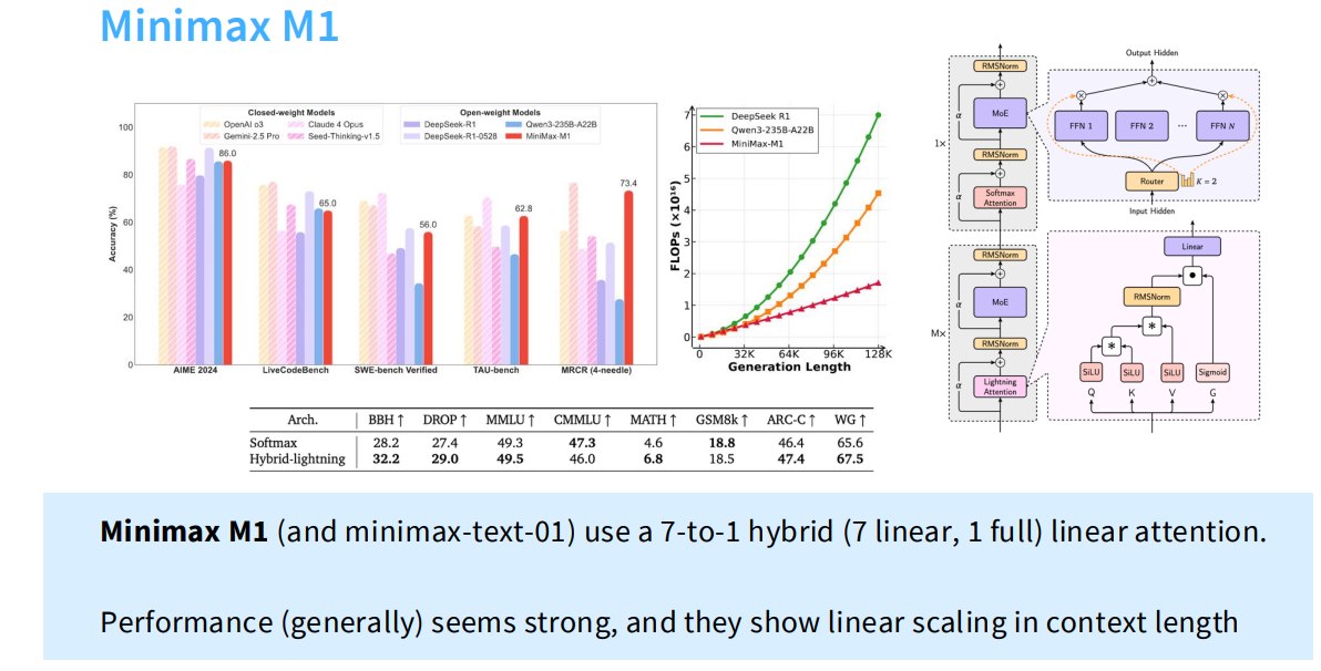
1.5 Minimax M1:linear + full attention hybrid
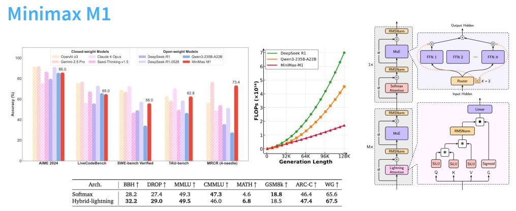
Minimax M1 和 minimax-text-01 使用:
- 7 层 linear attention
- 1 层 full attention
这样的混合设计有一个直觉:
- 线性注意力提供长上下文推理效率;
- full attention 保留强表达能力和全局精确交互。
linear scaling in context length
即上下文长度增长时,成本近似线性增长。同时性能看起来也比较强。
1.6 从 Linear Attention 到 Mamba-2
线性注意力状态更新是:
$$ S_t = S_{t-1} + k_t v_t^T $$输出:
$$ y_t = q_t^T S_t $$
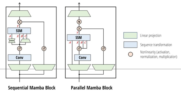
Mamba-2 的形式:
$$ S_t = γ_t S_{t-1} + k_t v_t^T $$输出:
$$ y_t = q_t^T S_t + v_t^T D $$其中:
$$ γ_t = f(x_t) $$也就是说,衰减系数 $γ_t$ 不是固定的,而是由当前输入决定的。
这就是一种 gating:当前 token 可以决定保留多少历史状态。
Q:为什么说 gating is good.
A:
门控机制在很多地方都有效:
- LSTM / GRU 中的门控;
- SwiGLU 中的 gating;
- Mamba 中控制状态更新;
- Gated Delta Net 中选择性写入和擦除。
对于序列模型,gating 允许模型决定:
- 哪些信息应该记住
- 哪些信息应该忘掉
- 当前输入是否应该写入状态
这比简单累加状态更强。
Mamba-2 仍然保留 duality:
- 训练时可以并行计算;
- 推理时可以递推更新状态。
1.7 Nemotron 3:Mamba-Attention Hybrid
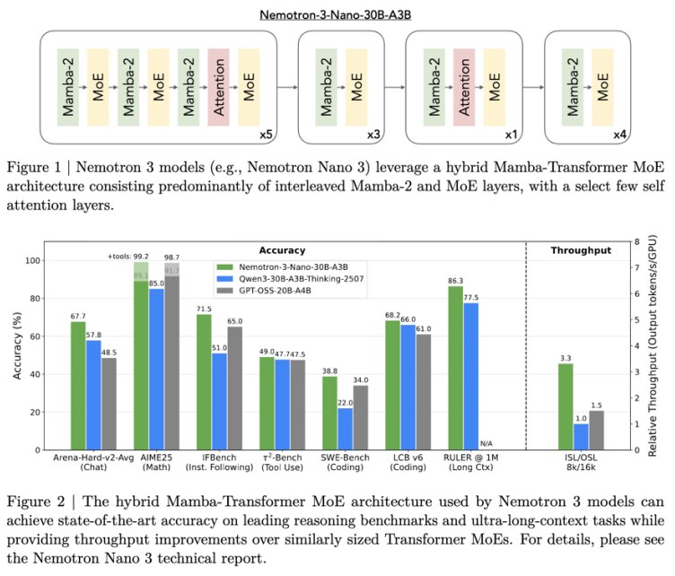
讲义提到 Nemotron 3 使用 Mamba attention hybrid:多数层使用 Mamba/线性或状态空间类模块,少数层使用标准 attention。
讲义说它和类似模型相比性能 comparable 或更好。
这说明当前趋势之一是:
不一定完全替代 attention,而是用 hybrid architecture 在效率和性能之间折中。
1.8 Gated Delta Net
讲义接下来介绍比 Mamba-2 更进一步的泛化:Gated Delta Net,GDN:
$$ S_t = γ_t (I - β_t k_t k_t^T) S_{t-1} + β_t k_t v_t^T $$输出:
$$ y_t = q_t^T S_t $$其中:
$$ γ_t = f(x_t) \\ β_t = f(x_t) $$当 $β_t = 0$ 时,那么当前输入不写入状态,只做衰减。
$$ S_t = γ_t S_{t-1} $$也就是说,模型可以选择:当前 token 不要更新记忆。
值得注意的是,GDN 还有一项:
$$ (I - β_t k_t k_t^T) S_{t-1} $$$k_t k_t^T$ 这个秩1矩阵表示在当前 key 方向上选择性擦除旧状态。
直观理解:
如果当前输入带来了某个 key 方向的新信息,模型可以先擦掉旧状态中这个方向的信息,再写入新的 $k_t v_t^T$。
1.9 Qwen 3.5 / Qwen Next:GDN + Attention Hybrid
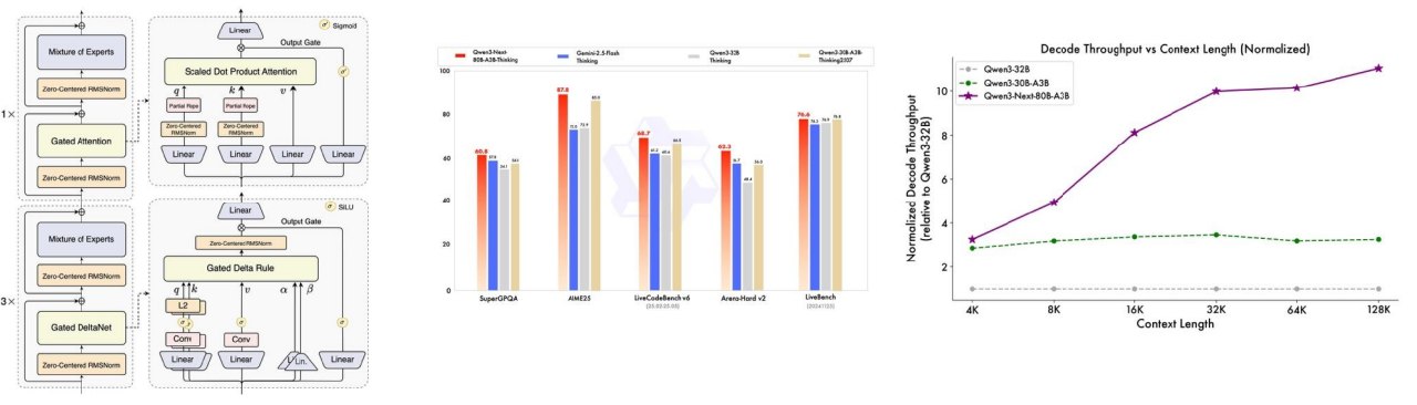
Qwen3.5 系列采用:3-to-1 GDN / Attention hybrids
也就是:
- 3 层 GDN
- 1 层 Attention
这种设计保留了 attention 的强表达能力,同时利用 GDN 改善推理效率和长上下文特性。
pretty reasonable performance with good inference characteristics
也就是说,这类 hybrid 架构在性能和推理效率之间取得了不错平衡。
1.10 Hybrid performance:混合架构效果
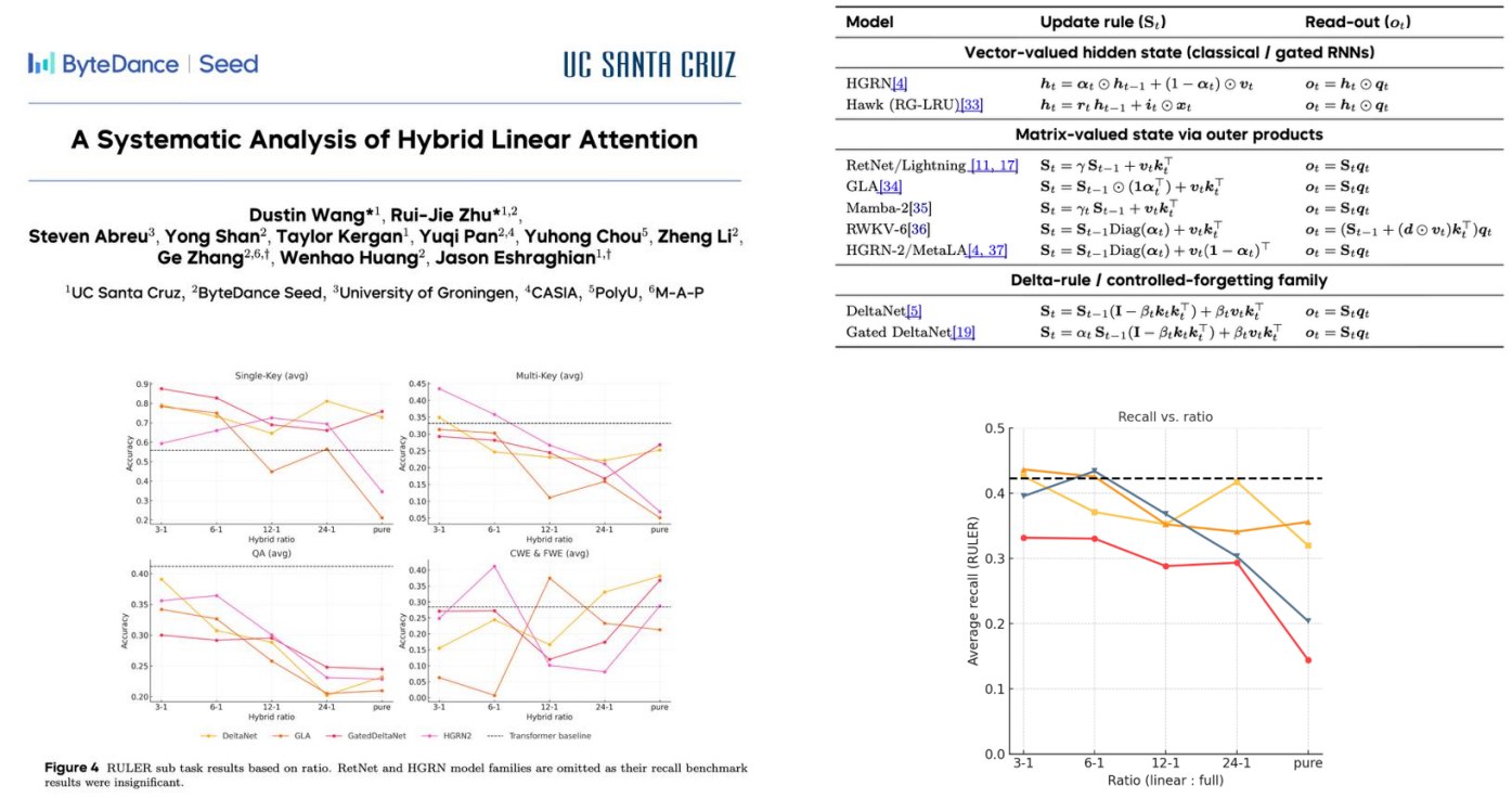
Not many controlled ablations, but some evidence of low losses at small hybrid ratios.
- 目前控制变量很严格的消融实验不多;
- 但已有证据表明,较小比例的 full attention 混入 linear/SSM/GDN 模块,就能达到较低 loss。
这说明一个趋势:完全替代 attention 可能很难,但少量 attention + 大量高效替代模块可能是很有前景的路线。
1.11 Sparse Adaptation:稀疏注意力作为另一条路线
除了 hybrid linear attention / Mamba / GDN,还有一种路线:Sparse Attention
Instead of attending to every token, do sparse attention.
也就是不要让每个 token attend 到所有 token,而是选择一部分重要 token。
1.12 DSA:D0 Sparse Attention
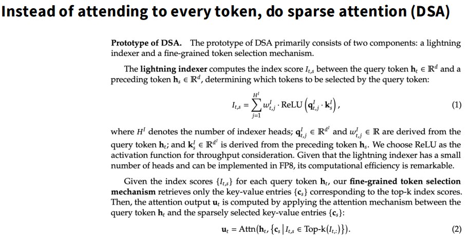
相关模型包括:
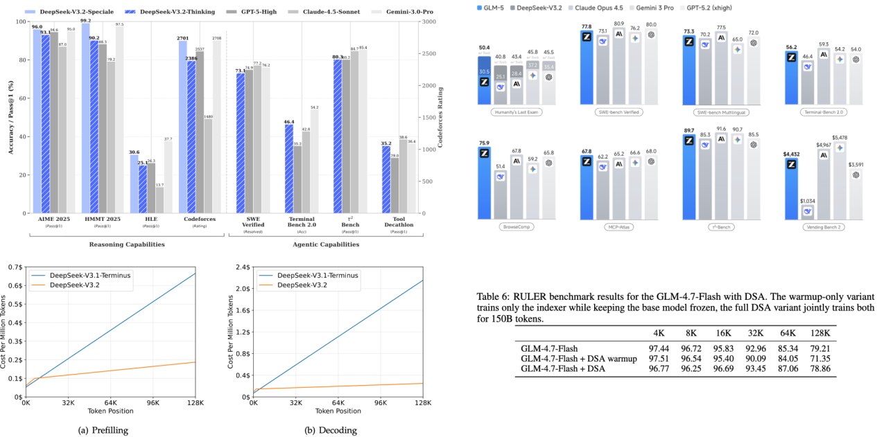
- DeepSeek v3.2;
- GLM5。
核心思想是:用一个轻量级 indexer 选择要 attend 的 token,从而减少 attention 成本。
如果 indexer 足够轻,整体可以获得显著收益。
讲义说 DSA 可以:post hoc adapted after dense short context pretraining
即,可以先训练一个短上下文 dense attention 模型,再后期适配成稀疏长上下文模型。
这很实用,因为从头训练长上下文模型成本很高。
二、Mixture of Experts,MoE
这节课剩下的篇幅都在讲 MoE。
MoE 是当前大模型发展中非常重要的路线。
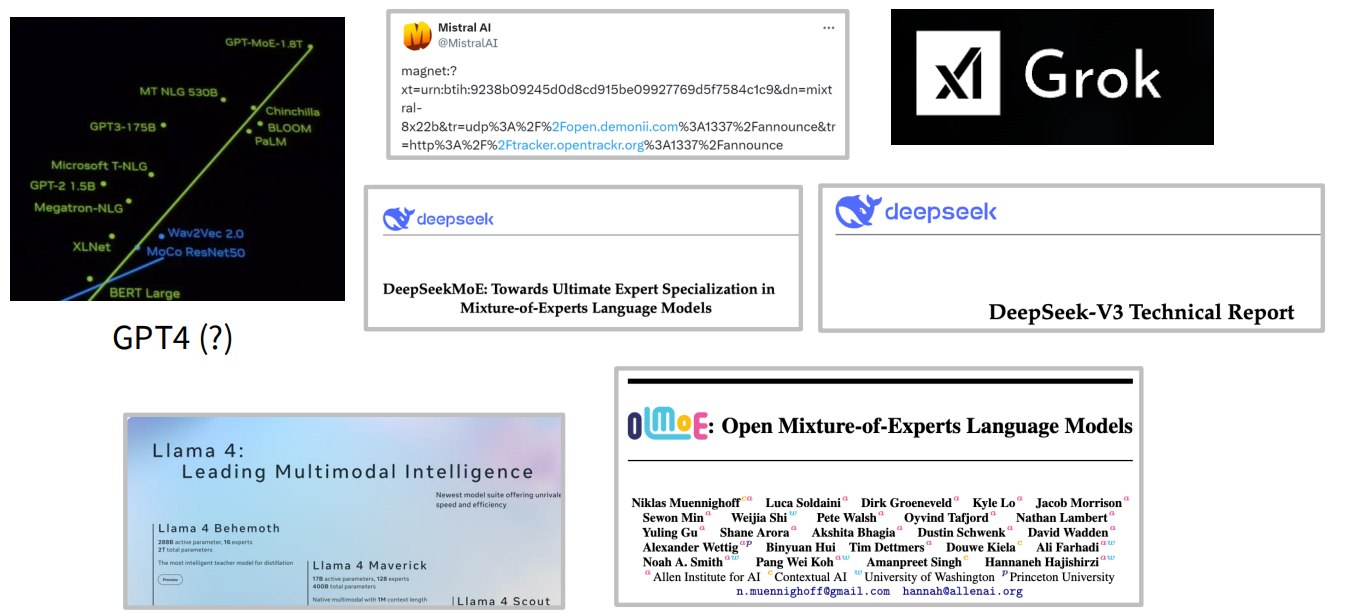
代表模型包括:
- Switch Transformer;
- GShard;
- Mixtral;
- DBRX;
- Grok;
- Qwen MoE;
- DeepSeek MoE;
- DeepSeek v3;
- Llama 4 Maverick 等。
2.1 什么是 MoE?
Replace big feedforward with many big feedforward networks and a selector layer.
也就是说,把 Transformer 里的 MLP / FFN 层替换成多个专家网络:
Expert 1: FFN
Expert 2: FFN
Expert 3: FFN
...
Expert N: FFN
然后用一个 router / gating network 为每个 token 选择其中一小部分 expert。
2.1.1 Dense FFN vs MoE FFN
普通 dense Transformer:每个 token 都经过同一个 MLP
MoE Transformer:每个 token 只经过少数几个专家 MLP
例如:
- 总共有 64 个 experts
- 每个 token 只激活 top-2 experts
MoE 虽然把原来单个MLP换成了多个 Expert MLP,增大了模型参数,但是通过控制每个token只经过少数几个Expert,其实FLOPs没有增加很多。
2.1.2 MoE 的关键优势
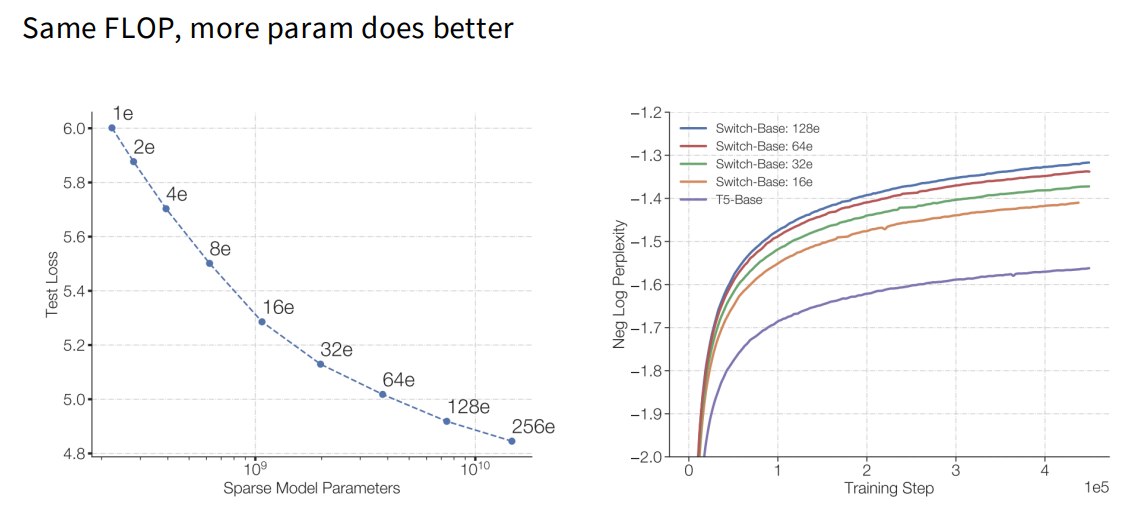
You can increase the # experts without affecting FLOPs.
如果每个 token 始终只激活固定数量的专家,比如 top-2,那么你可以增加总 expert 数量:
8 experts → 64 experts → 256 experts
总参数增加很多,但每个 token 使用的 expert 数不变,因此 FLOPs 变化不大。
这就是 MoE 的核心吸引力:同样 FLOPs,下拥有更多参数容量。
2.1.3 为什么MoE 越来越流行?
在相同计算量下,更多参数通常能带来更强能力:
MoE 可以更快训练到较好效果:
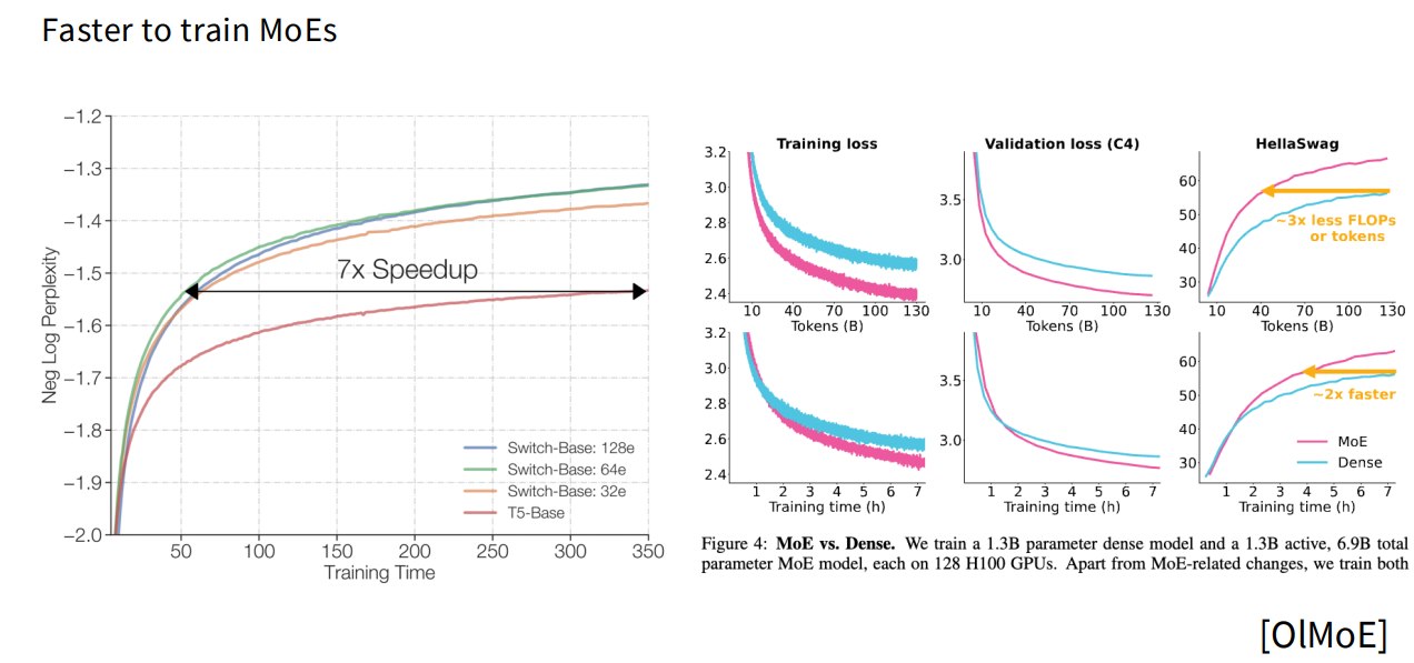
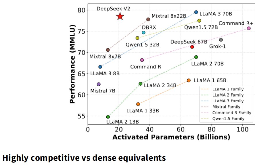
与相同训练预算或推理预算下的 dense 模型相比,MoE 常常更强:
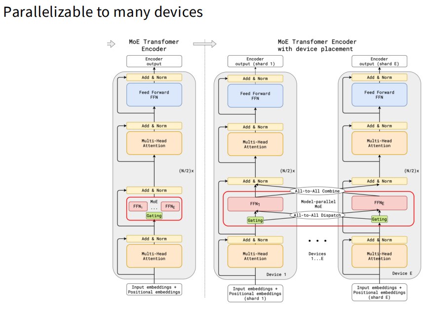
专家可以分布在不同 GPU / 节点上:
当然,这也带来通信复杂度,后面会讲。
2.1.4 为什么 MoE 没有更早全面流行?
1、Infrastructure is complex
MoE 需要复杂基础设施:
- expert parallel;
- token dispatch;
- all-to-all communication;
- load balancing;
- sparse matrix multiplication;
- expert capacity;
- token dropping。
这比 dense Transformer 难实现得多。
2、优势主要体现在 multi-node
MoE 的优势常常需要很多设备才能体现。
在单机小规模训练中,MoE 的通信和调度开销可能抵消收益。
3、Training objectives heuristic and sometimes unstable
MoE 路由是离散选择。
例如:选择 top-k experts
这本身不可微。
一般这种做离散选择的都表现为阶跃函数,导数不存在,没法梯度下降。
训练时通常用一些 heuristic balancing losses,这些损失不是特别优雅,也可能带来不稳定。
2.1.5 MoE 通常替换哪里?
Typical: replace MLP with MoE layer.
大多数 MoE 模型替换 Transformer block 中的 MLP(图左)。
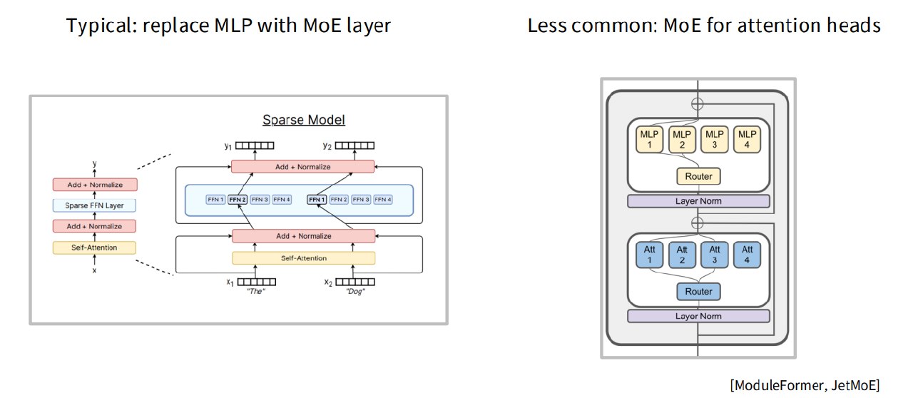
不太常见的是MoE for attention heads(图右)
主流还是:MoE 替换 FFN / MLP
2.2 MoE 怎么工作
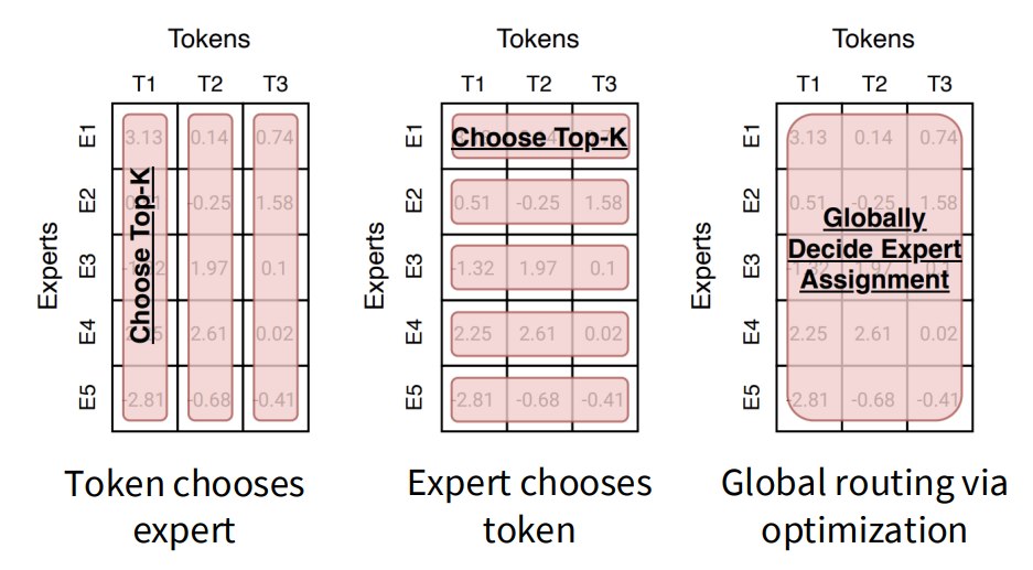
2.2.1 Routing function:路由函数
对每个 token,决定送给哪些 experts。
routing algorithm 可以归结为:choose top-k
2.2.2 Top-k routing
对于每个 token hidden state:$h_t$
router 计算每个 expert 的打分:$score_i = router_i(h_t)$
然后选择打分最高的 k 个 experts:$top-k experts$
再把 token 发送给这些 experts,最终输出通常是这些 expert 输出的加权和。
哪些模型用 top-k?
讲义列了很多:
| 模型 | k |
|---|---|
| Switch Transformer | 1 |
| GShard | 2 |
| Grok | 2 |
| Mixtral | 2 |
| Qwen | 4 |
| DBRX | 4 |
| DeepSeek | 7 或 8 等 |
这说明 top-k routing 是事实标准。
Router 打分方式
讲义提到:
- DeepSeek v1-v2 使用 logistic regressor 风格 router;
- Grok、Qwen 也类似;
- Mixtral、DBRX、DeepSeek v3 在 TopK 后做 softmax。
大致形式:
scores = W_router h
selected = topk(scores)
weights = softmax(scores[selected])
output = Σ weights_i Expert_i(h)
有些模型使用 sigmoid gate,有些使用 softmax。
2.2.3 Hashing、RL、Linear Assignment 等路由
1、Hashing
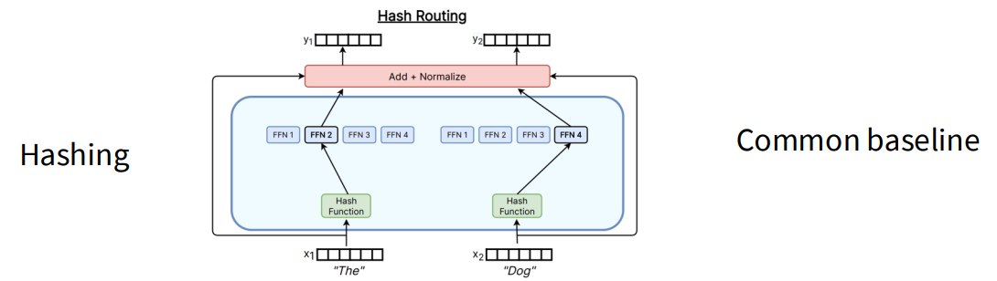
Hashing routing 是一个常见 baseline。用哈希规则把 token 分到 expert。
优点:
- 简单;
- 负载容易控制。
缺点:
- 不够自适应;
- 表达能力弱。
2、RL routing
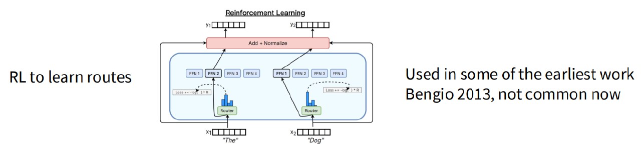
早期有用强化学习学习 routing policy 的方法。
理论上 RL 更适合离散决策。
但讲义说:
RL is the right solution but gradient variances and complexity means it’s not widely used.
也就是:
- 理论上合理;
- 实践中梯度方差大;
- 系统复杂;
- 性能收益不够稳定。
所以现代 MoE 不太用 RL routing。
2.2.4 Linear assignment routing
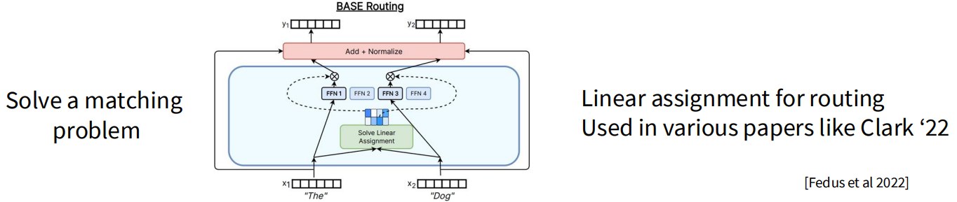
有些论文把路由看成 matching problem。
例如:在 tokens 和 experts 之间求一个全局匹配
-
优点是可以全局平衡。
-
缺点是优化和实现复杂。
主流大模型依然使用简单 top-k。
2.3 Expert 设计:数量、激活数量、共享专家、细粒度专家
MoE 不只是 router,expert 配置也很重要。
讲义列了很多模型的 expert 设置:
| 模型 | Routed experts | Active experts | Shared experts | Fine-grained ratio |
|---|---|---|---|---|
| GShard | 2048 | 2 | 0 | - |
| Switch Transformer | 64 | 1 | 0 | - |
| Mixtral | 8 | 2 | 0 | - |
| DBRX | 16 | 4 | 0 | - |
| Grok | 8 | 2 | 0 | - |
| DeepSeek v1 | 64 | 6 | 2 | 1/4 |
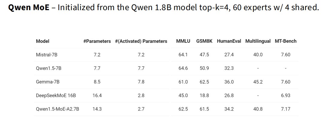
| Qwen 1.5 | 60 | 4 | 4 | 1/8 |
| DeepSeek v3 | 256 | 8 | 1 | 1/14 |
| OlMoE | 64 | 8 | 0 | 1/8 |
| MiniMax | 32 | 2 | 0 | ~1/4 |
| Llama 4 Maverick | 128 | 1 | 1 | 1/2 |
2.3.1 Routed experts
Routed experts 是由 router 选择的专家。
例如:DeepSeek v3: 256 routed experts
每个 token 从中选择一部分。
2.3.2 Active experts
Active experts 是每个 token 实际激活的专家数。
例如:DeepSeek v3: active = 8
表示每个 token 会经过 8 个 routed experts。
2.3.3 Shared experts
Shared experts 是始终激活的专家。
讲义提到 DeepSeek / Qwen 等会有:
shared experts that are always on
例如 DeepSeek v1 有 2 个 shared experts。
直觉是:
某些通用能力应该被所有 token 使用,不应该完全依赖路由选择。
所以 shared expert 提供一条稳定通用路径。
2.3.4 Fine-grained experts
Fine-grained expert 是把专家做得更小、数量更多。
例如把一个大 expert 切成多个小专家。
好处可能是:
- 路由更细;
- 专家专门化更强;
- 激活组合更灵活。
讲义提到 DeepSeek 和 OlMoE 都讨论过 fine-grained experts。
但实验结论不完全一致:
- DeepSeek paper:更多 experts 和 shared experts 一般有帮助;
- OlMoE:fine-grained experts 有收益,但 shared experts 没有收益。
所以 shared expert 是否有用还取决于设置。
2.4 MoE 训练
2.4.1 核心难点
Major challenge: we need sparsity for training-time efficiency, but sparse gating decisions are not differentiable.
也就是说我们想让每个 token 只激活少数 experts:top-k sparse routing
这样训练才省计算,但 top-k 是离散操作,不可微,因此训练 router 很困难。
2.4.2 解决方案
2.4.2.1 Reinforcement learning
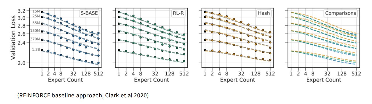
强化学习可以优化离散路由。
例如 REINFORCE。
讲义说:
RL via REINFORCE does work, but not so much better that it’s a clear win.
问题:
- 梯度方差高;
- 实现复杂;
- 训练不稳定;
- 收益不够明显。
所以不是主流。
2.4.2.2 Stochastic approximations
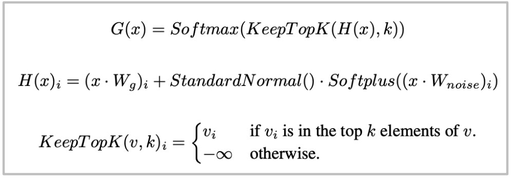
早期 Shazeer et al. 2017 使用 stochastic routing。
做法是:给 routing score 加高斯扰动
让路由决策带随机性。
好处:
- expert 更鲁棒;
- softmax 让模型学习如何排序专家;
- 减少专家过早固定和脆弱 specialization。
Switch Transformer / Fedus et al. 也使用过 stochastic jitter,例如 uniform multiplicative perturbation。
但讲义说后续 Zoph et al. 2022 移除了这种 jitter。
2.4.2.3 Heuristic balancing losses
为什么需要负载均衡?
如果没有约束,router 可能把大量 token 都送给少数几个 expert。
这会导致:
- 计算不均衡;
- 某些 GPU 过载;
- 其他 expert 没训练到;
- token dropping;
- 系统效率很差。
所以 MoE 需要让 experts 被相对均匀使用。
Switch Transformer 的 balancing loss
讲义提到 Switch Transformer 中的 heuristic balancing loss。
核心思想是:如果某个 expert 被使用太频繁,就在损失中惩罚它,让 router 降低它的概率。
讲义提到:more frequent use = stronger downweighting
也就是说,被选得越多的 expert,会受到更强负反馈。
这样 router 会被鼓励使用其他 experts。
DeepSeek v1-v2 的 balancing
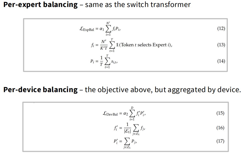
DeepSeek v1-v2 有:
- Per-expert balancing
- 类似 Switch Transformer,让每个 expert 使用更均匀。
- Per-device balancing
- 不仅平衡 expert,还按设备聚合,平衡每个设备上的负载。
为什么需要 device balancing?
因为 expert 分布在不同 GPU 上。
如果某些 GPU 上的 experts 被大量选中,那些 GPU 就会成为瓶颈。
所以要平衡:
- expert-level load
- device-level load
讲义说 DeepSeek v3 使用:per-expert biases,并用 online learning 调节这些 bias。
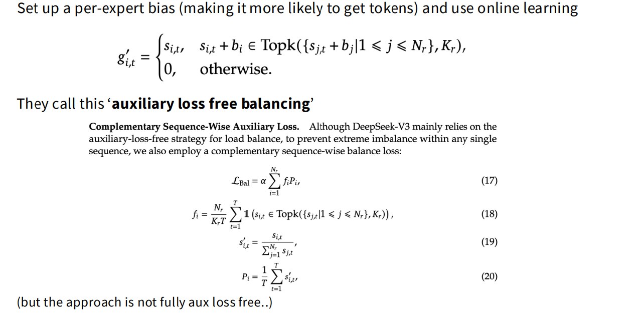
思想是:
给每个 expert 一个可调整偏置,让使用少的 expert 更容易被选中,使用多的 expert 更不容易被选中。
这被称为:
auxiliary loss free balancing
但讲义也提醒:
the approach is not fully aux loss free.
因为 DeepSeek v3 仍有 seq-wise aux 等机制,所以不是完全没有辅助项。
2.4.3 MoE 的系统侧训练问题
MoE 在系统上既有优势,也有复杂性。
1、Expert parallelism
每个 expert 是一个 FFN,可以放在不同设备上。
例如:
GPU 0: Expert 0,1,2,3
GPU 1: Expert 4,5,6,7
...
这样模型参数可以横向扩展到许多设备。
2、Token dispatch 和 all-to-all communication
每个 token 需要根据 router 被发送到对应 expert 所在设备。
这会导致通信:
tokens → experts
experts output → original token order
通常需要 all-to-all。这在多节点训练中非常复杂。
3、Sparse matrix multiplication
由于每个 expert 只处理部分 tokens,计算是不规则的。
现代库如:
MegaBlocks
会使用更聪明的 sparse matrix multiplication 来提高效率。
讲义提到 MegaBlocks 被许多 open MoE 使用。
4、Nemotron 3 的通信优化
讲义提到 Nemotron 3 的一个新想法:
down-projecting the activations to reduce communication.
也就是说,在跨设备传 token 激活时,先把激活降维,减少通信量。这体现了 MoE 中通信成本的重要性。
2.4.4 MoE 的随机性问题
MoEs can have additional stochasticity beyond normal models.
为什么?
因为 token dropping / routing 可能发生在 batch level。
例如某个 expert 容量有限。
如果一个 batch 中太多 token 都选择同一个 expert,那么超出容量的 token 可能被丢弃或改路由。
这意味着:
你的 token 是否被 drop,可能取决于同一个 batch 里其他人的 token。
讲义说得很形象:
other people’s queries can drop your token!
这会导致 MoE 推理或训练有额外随机性,尤其在 serving 中需要小心。
2.4.5 MoE 稳定性问题
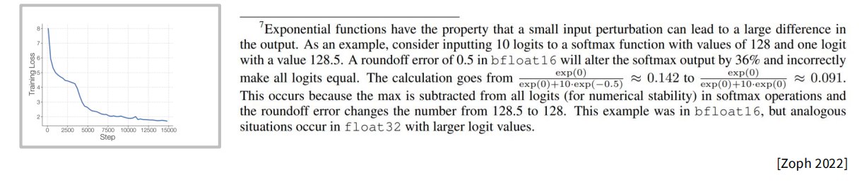
讲义说 MoE 的稳定性也需要特殊处理。
Router 用 FP32
一个常见解决方案:Use Float32 just for the expert router
即使主模型用 bf16/fp16,router 也用 float32。
因为 router logits 和 softmax/top-k 对数值误差敏感
Router z-loss
类似输出 softmax 的 z-loss,router 也可以加 z-loss。
目的:
- 防止 router logits 爆炸
- 稳定 expert 选择
2.4.6 MoE fine-tuning 问题
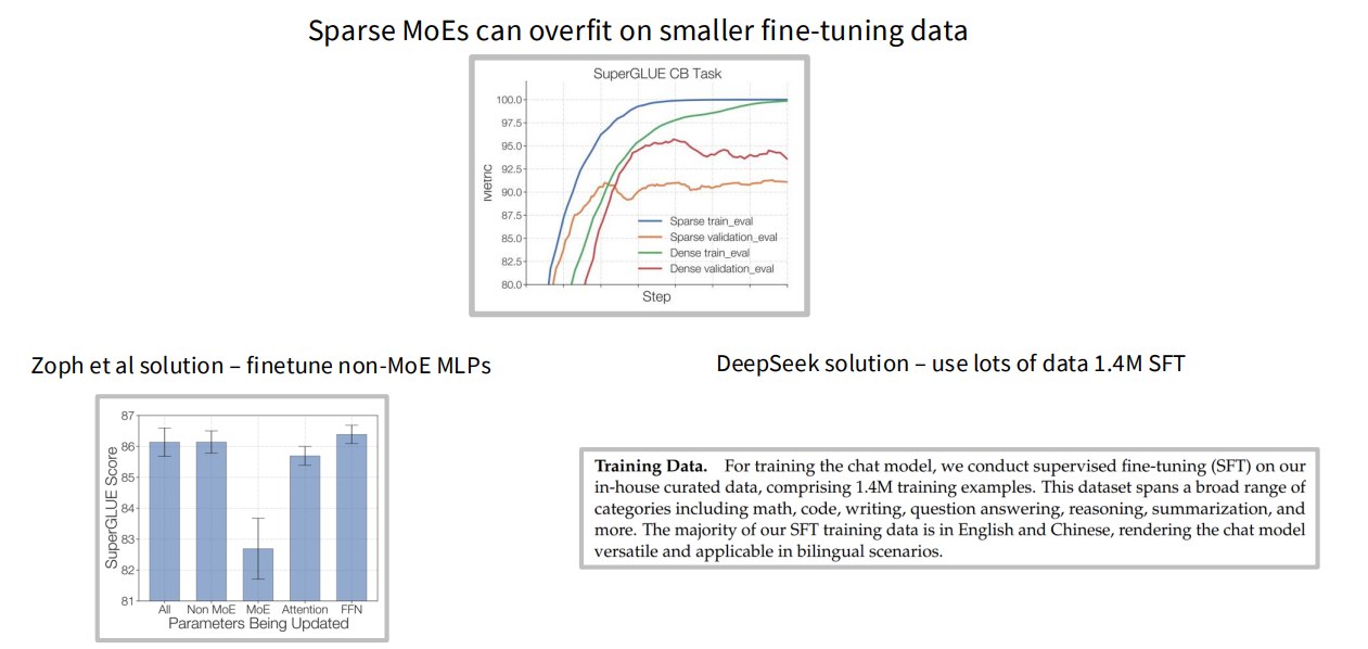
Sparse MoEs can overfit on smaller fine-tuning data.
原因可能是:
- 每个 expert 只看到部分 token;
- 小数据下某些 expert 更新稀疏;
- 路由分布容易变形;
- 容易过拟合。
解决方案例子:
1、Zoph et al. solution
finetune non-MoE MLPs
即 fine-tuning 时可能只调非 MoE 部分,减少过拟合。
2、DeepSeek solution
use lots of data
DeepSeek 使用大规模 SFT 数据,例如 1.4M SFT。讲义强调的是:MoE fine-tuning 小数据时不一定简单。
2.4.7 Upcycling:从 dense 模型初始化 MoE
Can we use a pre-trained LM to initialize a MoE?
这就是 upcycling。
假设你已经有一个 dense 模型。
MoE upcycling 做法是:
- 把 dense MLP 复制/拆分/扩展成多个 experts
- 然后继续训练 MoE
这样不用从头训练 MoE,可以继承 dense 模型能力。
不过Instructor在课程中提到,现在基本没人这么做,不如直接从头开始训练。
一些例子:
2.5 DeepSeek MoE v1/v2/v3 架构演进
讲义最后重点走了一遍 DeepSeek MoE 架构。
2.5.1 DeepSeek MoE v1
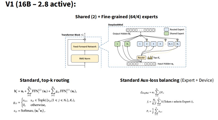
配置:
- 16B total parameters
- 2.8B active parameters
特点:
- 标准 top-k routing;
- shared experts = 2;
- fine-grained experts:64/4;
- standard auxiliary loss balancing;
- 包括 expert-level 和 device-level balancing。
可以理解为:
DeepSeek v1 是比较标准但带 shared + fine-grained experts 的 MoE。
2.5.2 DeepSeek MoE v2
配置:
236B total parameters
21B active parameters
新设计:
- shared experts = 2;
- fine-grained experts:160/10;
- active experts = 6;
- communication balancing loss;
- Top-M device routing。
Communication balancing loss:不仅平衡 expert 负载,还平衡通信:
communication in
communication out
Top-M device routing:不是只选 expert,也考虑 device。先选择若干设备,再在设备内选 experts,可以控制跨设备通信。
2.5.3 DeepSeek MoE v3
讲义中写:
671B total
37B active
特点:
- shared experts = 1;
- routed experts ≈ 258 或 256 级别;
- active experts = 8;
- sigmoid + softmax top-k + top-M;
- auxiliary-loss-free balancing;
- seq-wise aux。
DeepSeek v3 的核心趋势:
- 更多更细 experts
- 更复杂但更高效的路由和平衡
- 更强系统优化
2.6 DeepSeek v3 还需要什么?MLA
讲义 bonus 部分讲 DeepSeek v3 的 MLA:Multihead Latent Attention
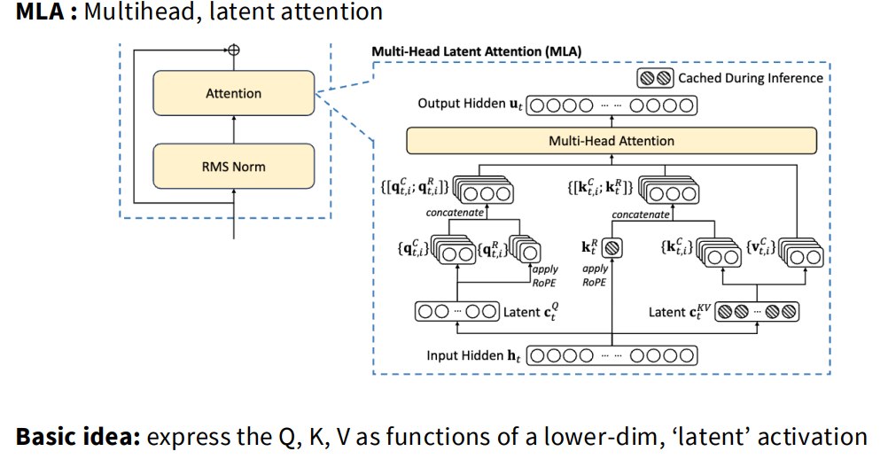
MLA 的基本想法
讲义说:
express the Q, K, V as functions of a lower-dim latent activation.
也就是把 Q/K/V 表示为一个低维 latent activation 的函数。
对于 KV cache,标准 Transformer 要存每层每个 token 的 K 和 V。
MLA 想改成只存低维 latent:$c_t^{KV}$
然后需要时从 latent 生成 K/V。
好处:KV cache 显著变小。
为什么 MLA 省 KV cache?
标准 KV cache 存:$K_t, V_t$
每个 token、每层都要存一大堆向量。
MLA 存:$c_t^{KV}$
这是更低维的 latent。
然后:$K_t = W_UK c_t^{KV} V_t = W_UV c_t^{KV}$
这样推理时内存占用降低。
讲义说:
W_UK can be merged into the Q projection.
也就是某些矩阵可以合并,进一步优化计算。
MLA 和 RoPE 的冲突
讲义提到一个复杂点:RoPE conflicts with MLA-style caching.
没有 RoPE 时:
$$ Q = h W_Q\\ K = W_UK c_t^{KV} $$attention 内积:
$$因此可以把 $W_UK$ 合并进 Q projection。
但有 RoPE 时:
$$ Q_{rot} = h W_Q R_q\\ K_{rot} = R_k W_{UK} c_t^{KV} $$内积中间夹着旋转矩阵:
$$ h W_Q R_q R_k W_{UK} $$由于 RoPE 位置相关,不能简单合并。
解决方案:
Have a few non-latent key dimensions that can be rotated.
也就是保留一部分非 latent 的 key 维度专门用于 RoPE 旋转。
这就是 DeepSeek MLA 的一个关键工程/架构折中。
2.7 DeepSeek v3 还需要什么?MTP
讲义还提到:MTP: Multi-Token Prediction
基本想法:
用小型轻量模型预测多个未来 token。
这类似 EAGLE 一类 speculative / multi-token prediction 思路。
讲义说 DeepSeek v3 实际只做:one token ahead
也就是预测未来一步。
MTP 可以作为辅助训练目标,帮助模型学习更强的未来预测能力,也可能服务于推理加速。
讲义没有详细展开,建议读 DeepSeek v3 论文看消融。
2.6 MoE 总结
讲义最后总结:
- MoE 利用稀疏性
- 并不是每个输入都需要完整模型参数。
- 离散路由很难
- top-k 这种启发式方法却在实践中很有效。
- 经验结果已经非常充分
- MoE 现在确实有效,而且 cost-effective。
可以浓缩为:
MoE 用“只激活部分专家”的方式,让模型拥有超大参数容量,但每个 token 的计算量保持可控。

说些什么吧!