
零、写在前面
这一节讲了很多LLM并行训练的策略,难哭了。
一、LLM 网络与 collective communication 基础
1.1 为什么单 GPU scaling 不够
1.1.1 Compute 限制
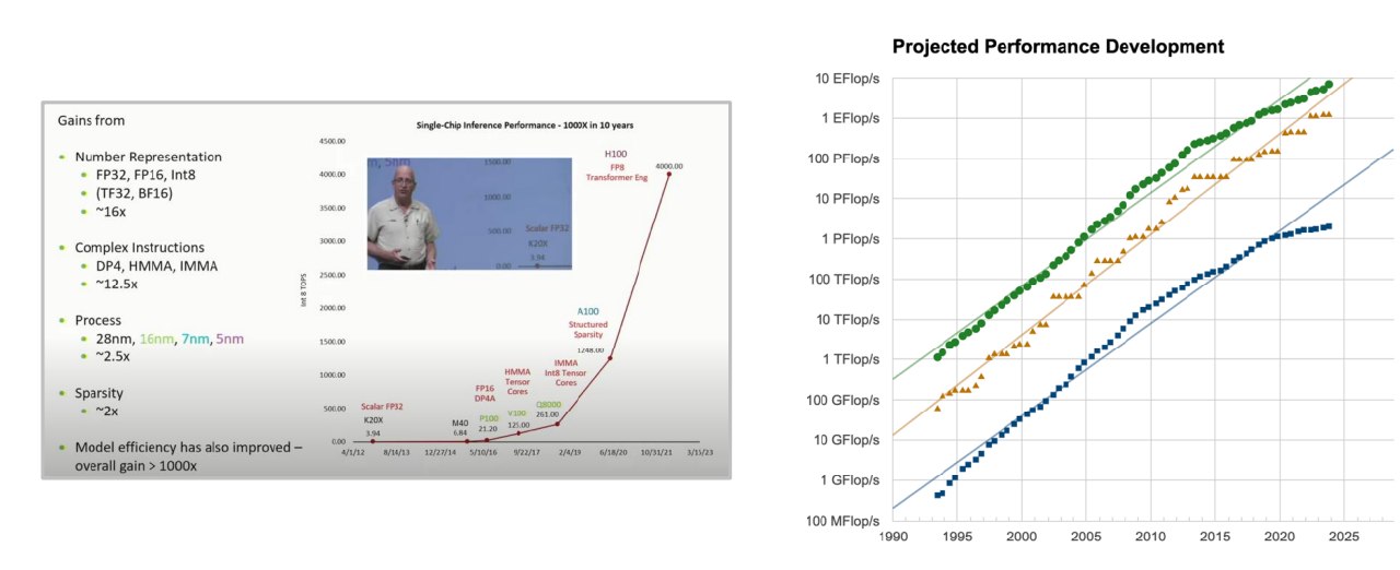
单张 GPU 的 FLOPs 有上限。大模型训练需要的总计算量通常可以粗略写成:
$$ \text{training FLOPs} \approx 6ND $$其中:
- N:模型参数量。
- D:训练 token 数。
这个近似来自 dense Transformer 训练中 forward + backward 的计算量估算。参数越多、token 越多,训练需要的总 FLOPs 越大。即使单 GPU 很强,训练时间也可能不可接受。
1.1.2 Memory 限制
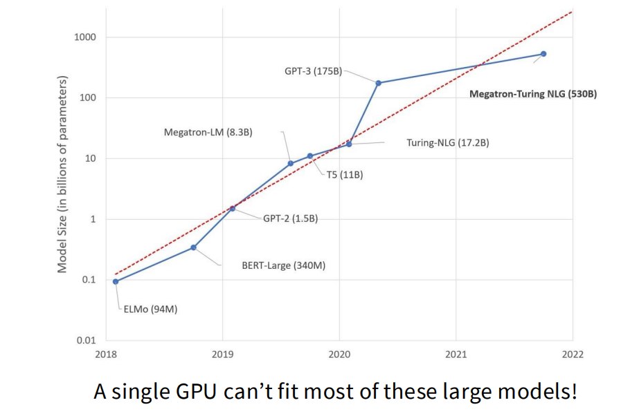
模型也越来越大。单 GPU 不只要放参数,还要放:
- parameters
- gradients
- optimizer states
- activations
- temporary buffers
- KV cache,尤其在长上下文训练/推理中
如果只看参数,BF16 参数每个 parameter 2 bytes。一个 70B 模型仅参数就约:
$$ 70 \times 10^9 \times 2 \approx 140\text{ GB} $$这已经超过许多单卡显存。训练时还要额外保存梯度、optimizer state 和激活,显存压力更大。
1.1.3 多 GPU、多机器的目标
多 GPU 的目标有两个:
- Memory scaling:把参数、梯度、optimizer state、激活分散到多张 GPU 上。
- Compute scaling:让更多 GPU 同时做有效计算,提高吞吐。
理想情况是:
$$ \text{max model size} \propto \#\text{GPUs} $$并且:
$$ \text{training throughput} \propto \#\text{GPUs} $$现实情况是:通信和同步会破坏线性 scaling。
1.2 Collective Communication 基础
这一部分其实就是对于lecture07的回顾。
1.2.1 常用 collective operations
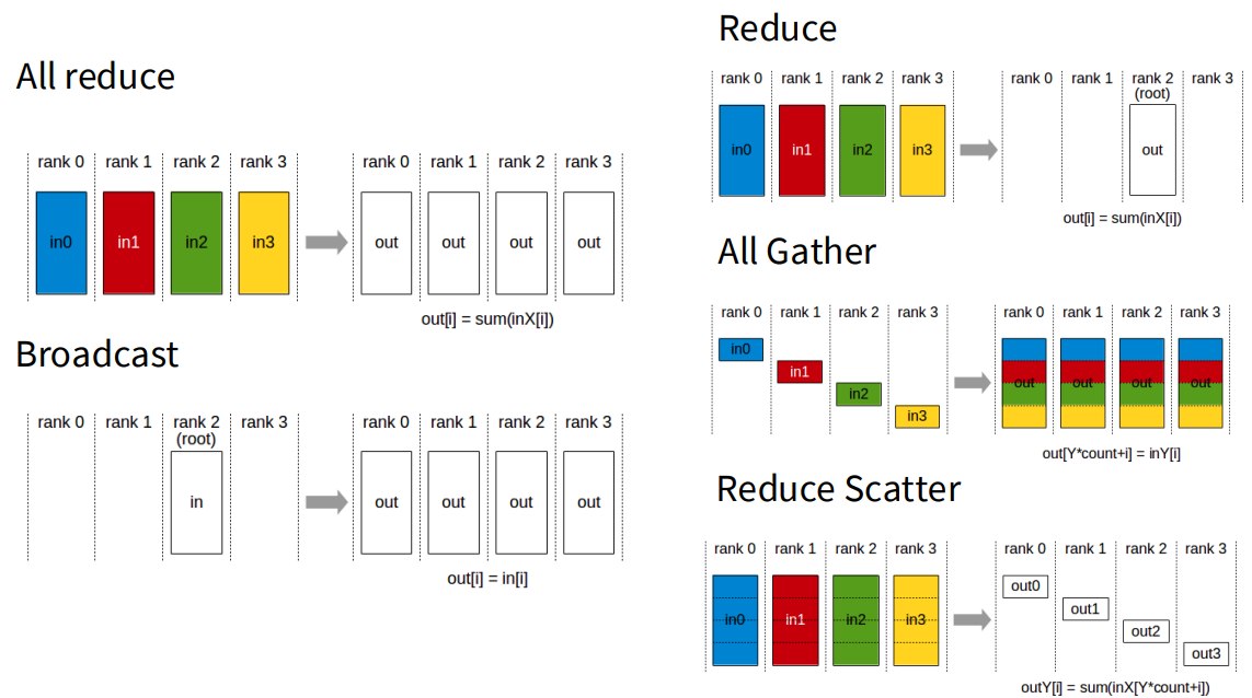
训练系统最常用的 collective 包括:
broadcastreduceall_reduceall_gatherreduce_scatterall_to_all
它们的角色可以这样记:
| 操作 | 直觉 | 训练中的典型用途 |
|---|---|---|
| broadcast | 一个 rank 发给所有 rank | 广播 checkpoint/参数 |
| all-reduce | 所有 rank 归约后每个 rank 都得到完整结果 | DDP 梯度同步 |
| reduce-scatter | 归约后每个 rank 只拿一片 | ZeRO/FSDP 梯度分片 |
| all-gather | 每个 rank 的 shard 拼成完整 tensor,并发给所有 rank | FSDP forward 前收集参数 |
| all-to-all | 每个 rank 给每个 rank 发一片 | MoE token dispatch |
1.2.2 All-reduce 与 reduce-scatter + all-gather
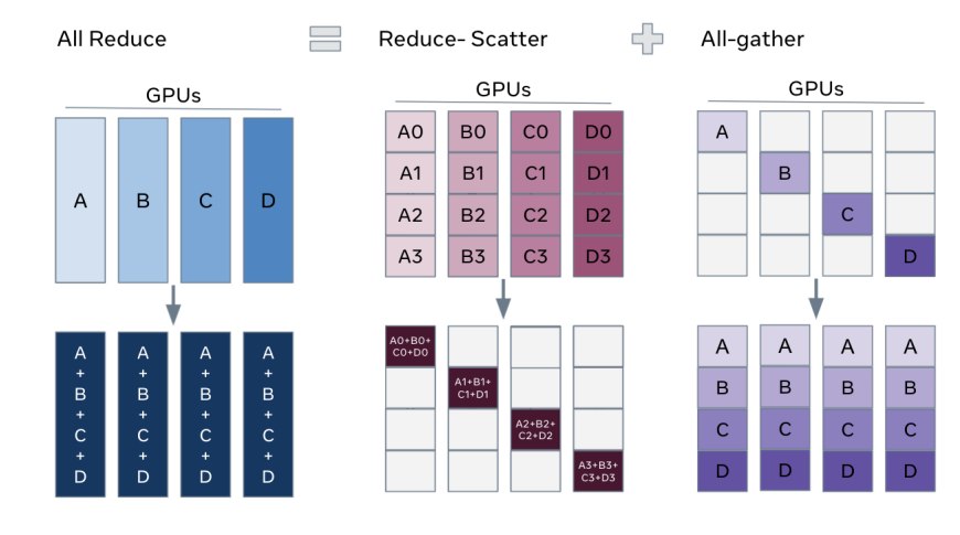
Reduce can be implemented as two steps: reduce-scatter and all-gather.
也就是:
$$ \text{all-reduce} = \text{reduce-scatter} + \text{all-gather} $$这个分解非常重要,因为 ZeRO/FSDP 正是利用它来减少显存占用。
教学伪代码:
# Every rank has a full gradient vector grad_r.
# all_reduce gives every rank the full summed gradient.
dist.all_reduce(grad, op=dist.ReduceOp.SUM)

# Equivalent conceptual decomposition:
grad_shard = reduce_scatter_sum(grad)
full_grad = all_gather(grad_shard)
为什么这有意义?因为有时我们不需要每个 rank 永远持有完整结果。比如 optimizer state 被分片后,每个 rank 只负责更新一部分参数,那么 reduce-scatter 后只保留梯度 shard 就够了。
1.3 TPU 网络 vs GPU 网络
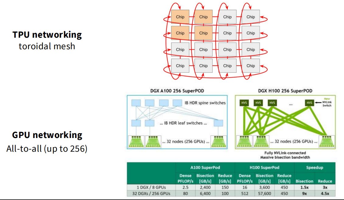
高层直觉:
- TPU 早期系统常见 mesh / torus 拓扑,适合规则通信模式。
- GPU 数据中心系统更强调 NVLink/NVSwitch、PCIe、InfiniBand、RoCE 等互联,以及较灵活的 all-to-all。
Mesh 的优势:
- 成本和布线相对可控。
- 对结构化通信,例如 tensor parallel 中固定 pattern 的通信,可以做得很快。
Tree / switch / all-to-all 风格拓扑的优势:
- 对不规则通信更友好。
- 对 MoE expert routing 这类 all-to-all 更自然。
1.4 为什么不把所有 GPU 都全互联
答案是系统工程上的成本、功耗、布线、交换芯片规模、故障域和拓扑复杂度。全互联的理论带宽诱人,但真实数据中心要在成本和可维护性之间折中。
所以大型训练通常形成层次化结构:
GPU 内部 HBM
-> 单节点 NVLink/NVSwitch
-> 节点间 InfiniBand/RoCE
-> 更大集群网络
并行策略也会顺着这个层次来设计:高频通信尽量放在节点内,低频或粗粒度通信才跨节点。
这节课的主讲还拿华为的卡跟navidia做了对比,华为更多的互联带来了更高的能耗。
1.5 小结
- 新的 compute unit 不再是一张 GPU,而是 datacenter。
- 多机器 scaling 想要:
- linear memory scaling
- linear compute scaling
- collective communication 是构建分布式训练系统的基础。
这也解释了为什么现代训练代码不只是模型代码,而是模型、并行策略、通信拓扑、调度和容错的组合。
二、标准 LLM 并行训练原语
下面主要展开:
- Data parallelism
- naive data parallel
- ZeRO stage 1-3
- Model parallelism
- pipeline parallel
- tensor parallel
- Activation parallelism
- sequence parallel
- context parallel
- Expert parallelism
2.1 Naive Data Parallelism
从最简单的 SGD 开始:
$$ \theta_{t+1} = \theta_t - \eta \sum_{i=1}^{B}\nabla f(x_i) $$如果有 M 台机器或 M 张 GPU,把 batch 切开:
$$ B_{\text{global}} = M \cdot B_{\text{local}} $$每个 rank 处理 B/M 个样本,计算本地梯度:
$$ g_r = \sum_{x_i \in \mathcal{B}_r}\nabla f(x_i) $$然后 all-reduce:
$$ g = \sum_{r=0}^{M-1} g_r $$最后每个 rank 用相同梯度更新相同参数。
伪代码:
for batch in dataloader:
    local_batch = shard_batch(batch, rank, world_size)

    loss = model(local_batch).loss
    loss.backward()

    for p in model.parameters():
        dist.all_reduce(p.grad, op=dist.ReduceOp.AVG)

    optimizer.step()
    optimizer.zero_grad()
2.1.1 Naive DP 的 compute scaling
优点:每张 GPU 只处理 batch 的一部分,所以计算可以随 GPU 数增加而增加。
限制:global batch 不能无限变大。大 batch 训练存在优化和泛化问题;当 M 接近或超过合适 batch size 时,继续加 GPU 会让每张 GPU 的 local work 太少,通信占比变高。
2.1.2 Naive DP 的通信开销
每个 step 都要同步梯度。对于参数量为 $P_{\text{param}}$ 的模型,梯度向量大小约等于参数量。Ring all-reduce 的通信量常粗略理解为:
$$ \text{traffic} \approx 2 \times \#\text{params} $$讲义里说 naive data parallel 每个 batch 传输约 $2\times\#\text{params}$,如果 batch 足够大,计算可以覆盖通信。
2.1.3 Naive DP 的显存问题
但其实真正糟糕的是 memory:每张 GPU 都复制完整模型状态。
混合精度 Adam 训练中,每个参数可能需要:
| 内容 | 典型 bytes/param |
|---|---|
| BF16/FP16 model parameter | 2 |
| BF16/FP16 gradient | 2 |
| FP32 master weight | 4 |
| Adam first moment | 4 |
| Adam second moment | 4 |
| 合计 | 16 |
所以 naive DP 的训练显存大约是:
$$ 16 \times \#\text{params} $$每个 rank 都要付这笔成本,没有 memory scaling。
2.2 ZeRO:解决 Data Parallel 的状态复制问题
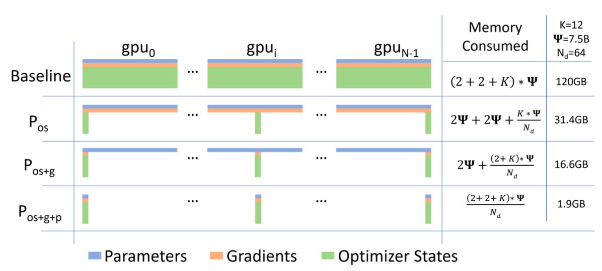
split up the expensive parts (state) and use the reduce-scatter equivalence.
ZeRO 的核心思想是:data parallel 仍然沿 batch 切数据,但不要让每个 rank 都保存完整 optimizer state、gradients、parameters。
令:
- N:参数数量。
- M:data parallel ranks 数。
- 每个参数训练状态约 16 bytes。
不同 ZeRO stage 逐步 shard 更多东西。
2.2.1 ZeRO Stage 1:Optimizer State Sharding
High-level idea:
- parameters:每个 rank 都有完整副本。
- gradients:每个 rank 都有完整副本。
- optimizer states:按 rank 分片。
每个 worker 负责更新一部分 parameters,对应它持有的 optimizer state shard。
如何工作?
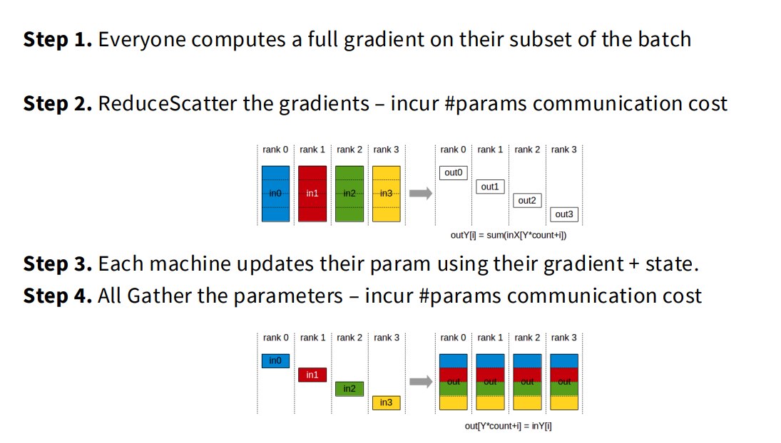
- 每个 rank 在自己的 batch shard 上计算完整梯度。
- 对 gradients 做 reduce-scatter,让每个 rank 得到自己负责参数的 gradient shard。
- 每个 rank 用自己的 optimizer state shard 更新对应参数 shard。
- all-gather 更新后的参数,让所有 rank 重新拥有完整参数。
2.2.2 ZeRO-1 通信与显存
和 naive DDP 对比:
| 方法 | 通信 primitive | 通信量 | 每 rank 显存直觉 |
|---|---|---|---|
| Naive DDP | gradients all-reduce | \(2N\) | 参数、梯度、optimizer 全复制 |
| ZeRO-1 | reduce-scatter gradients + all-gather params | \(2N\) | optimizer state 分片 |
讲义说 ZeRO-1 在 bandwidth-limited regime 中几乎是 free memory win,因为通信量和 all-reduce 同阶。
若用 K 表示 optimizer state bytes/param,粗略写法:
$$ \text{Naive DP memory} \approx (4 + K)N $$$$ \text{ZeRO-1 memory} \approx \left(4 + \frac{K}{M}\right)N $$这里的 4 可以理解为参数和梯度等未分片部分的近似 bytes/param。
2.2.3 ZeRO Stage 2:Gradient Sharding

High-level idea:
- optimizer state sharded。
- gradients 也 sharded。
- parameters 仍然 replicated。
关键难点:每个 rank 在 backward 时会产生完整梯度,但不能长时间 materialize 完整 gradient vector,否则显存又爆。
2.2.4 ZeRO-2 如何工作
- backward 沿 computation graph 逐层进行。
- 某层 gradient 一产生,就立刻 reduce 到负责该 shard 的 worker。
- 一旦该 gradient 不再需要,就释放。
- 每个 rank 用自己的 gradient shard 和 optimizer state shard 更新参数 shard。
- all-gather 参数。
伪代码:
for layer in reversed(model.layers):
    grad = compute_layer_grad(layer)

    # Do not keep the full gradient around.
    grad_shard = reduce_scatter_sum(grad)
    free(grad)

    if owns(layer, rank):
        update_with_sharded_optimizer(layer.param_shard, grad_shard)

full_params = all_gather(param_shards)
ZeRO-2 的实质是把通信插入 backward 过程,配合及时释放,降低 peak memory。
2.2.5 ZeRO Stage 3 / FSDP:Shard Everything
High-level idea:
-
parameters sharded。
-
gradients sharded。
-
optimizer states sharded。
-
forward/backward 需要某层参数时,临时 all-gather。
- 比如 rank0、rank1 分别负责batch0和batch1的前向过程,分别拿着layer0 和 layer1 的参数,那么再计算前向过程的时候二者在必要时是需要参数共享的。
-
用完后释放完整参数。
2.2.6 Baby version
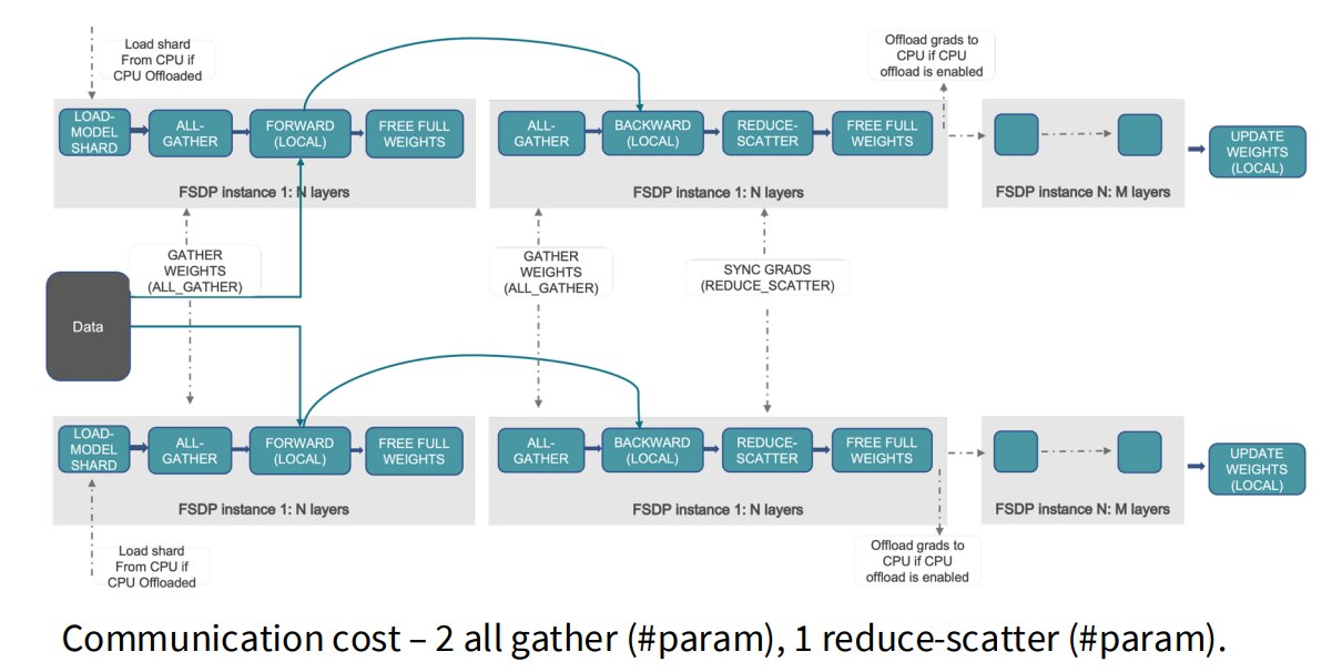
ZeRO-3 的通信成本大致是:
- 2 次 all-gather 参数。
- 1 次 reduce-scatter 梯度。
伪代码:
for block in model.blocks:
    # Forward: gather full parameters just in time.
    full_params = all_gather(block.param_shard)
    y = block.forward(x, full_params)
    free(full_params)

for block in reversed(model.blocks):
    # Backward may need parameters again.
    full_params = all_gather(block.param_shard)
    grad = block.backward(full_params)
    free(full_params)

    # Gradients are reduced and sharded.
    grad_shard = reduce_scatter_sum(grad)
    optimizer_step(block.param_shard, grad_shard, opt_state_shard)
2.2.7 Incremental communication / computation
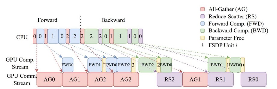
真实 FSDP/ZeRO-3 的关键思想:
- parameters 和 gradients 被 requested / sent 后立即释放。
- all-gather 可以和 forward computation overlap。
- reduce-scatter 可以和 backward computation overlap。
这也是 FSDP 不只是“把参数切开”那么简单。它是一种调度机制:尽量让通信发生在计算同时,减少 wall-clock overhead。
2.2.8 ZeRO stage 通信总结
| 方法 | 通信量直觉 | 显存收益 |
|---|---|---|
| DDP | $2\times\#\text{params}$ | 无 state sharding |
| ZeRO-1 | $2\times\#\text{params}$ | optimizer state sharding |
| ZeRO-2 | $2\times\#\text{params}$ | optimizer + gradients sharding |
| ZeRO-3 / FSDP | $3\times\#\text{params}$ 左右 | parameters + gradients + optimizer 全分片 |
ZeRO-3 通信多一些,但显存收益巨大。
2.2.9 ZeRO in practice:会不会 fit?
估算:如果除了 master weights 以外都用 BF16,约 12 bytes/param。
在 8 张 A100 80GB 上,粗略最大参数量:
| 方法 | 每 rank bytes/param 近似 | 最大模型参数量直觉 |
|---|---|---|
| Baseline | 12 | 约 6.7B |
| ZeRO-1 | 5 | 约 16B |
| ZeRO-2 | \(2 + 10/8\) | 约 24.6B |
| ZeRO-3 | \(12/8\) | 约 53.3B |
这里的重点不是具体数值,而是 scaling 方式:
$$ \text{ZeRO-3 memory per rank} \approx \frac{\text{full training state}}{M} $$这才是真正的 memory scaling。
2.2.10 剩余问题
1、Compute scaling 受 batch size 限制
Data parallel 通过扩大 global batch 来用更多 GPU:
$$ B_{\text{global}} = M \cdot B_{\text{local}} $$但 batch size 不能无限增大。训练质量、优化稳定性和吞吐都会出现 diminishing returns。
当机器数接近 batch size 或 local batch 太小,通信 overhead 会很高。
2、模型仍可能不 fit
ZeRO-1/2 主要 shard optimizer state 和 gradients,不 shard parameters,因此不一定能让巨大模型 fit。
ZeRO-3 shard parameters,但不直接解决 activation memory。对于长序列、深模型、大 batch,activation 仍可能是显存瓶颈。
所以我们需要 model parallelism 和 activation parallelism。
2.3 Model Parallelism:按模型切分
model parallelism 也像zero-3 那样切分参数,不过model parallelism 还进行激活值的通信。
本讲覆盖三种:
- Pipeline parallelism:沿 depth 切层。
- Tensor parallelism:沿 width 切矩阵。
- Expert parallelism:沿 experts 切 MoE。
2.3.1 Pipeline Parallelism:沿层切分
2.3.1.1 Layer-wise parallel 的问题
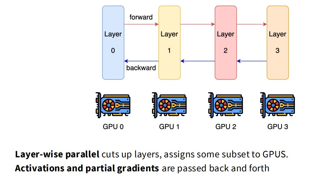
最直接的 layer-wise parallel:
GPU 0: layers 0..k
GPU 1: layers k+1..m
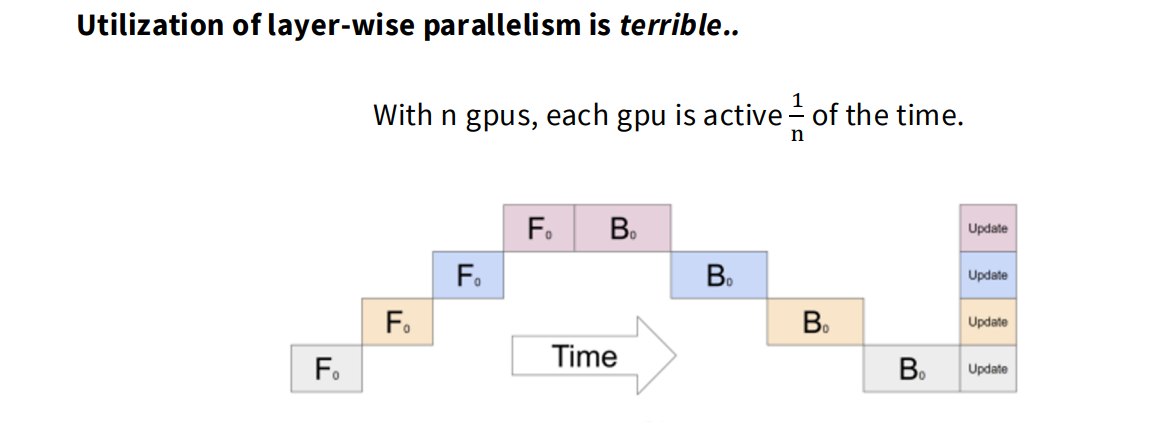
forward 时 GPU 0 先算,GPU 1 等。backward 反过来。若有 \(n\) 个 GPUs,每个 GPU 可能只有约 \(1/n\) 时间活跃,utilization 很差。
2.3.1.2 Micro-batch pipeline
解决方案:把 batch 切成 micro-batches,让 pipeline 中不同 stage 同时处理不同 micro-batch。
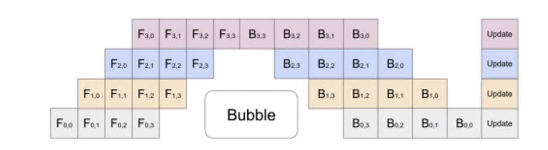
伪代码:
micro_batches = batch.chunk(num_micro_batches)

for t in range(num_micro_batches + num_stages - 1):
    for stage in stages:
        mb = schedule[t, stage]
        if mb is not None:
            activation = recv_from_prev(stage, mb)
            activation = stage.forward(activation)
            send_to_next(stage, mb, activation)
Pipeline bubble 的直观比例:
$$ \text{bubble ratio} \approx \frac{n_{\text{stages}} - 1}{n_{\text{micro}}} $$所以 micro-batches 越多,bubble 占比越小。但 micro-batch 太小会降低 matmul 效率,也可能增加调度开销。
2.3.1.3 为什么还要用 pipeline
pipeline 虽然有 bubble,但仍有价值:
- 相比 DDP,pipeline 可以节省参数显存。
- 相比 FSDP,pipeline 的通信取决于 activation 大小,而不是参数大小。
- pipeline 是 point-to-point communication,适合跨较慢网络链接。
激活通信量大致是:
$$ O(b \cdot s \cdot h) $$其中:
- b:micro-batch size。
- s:sequence length。
- h:hidden size。
这通常比频繁跨节点做 tensor all-reduce 更容易接受。
2.3.1.4 高级 pipeline schedule
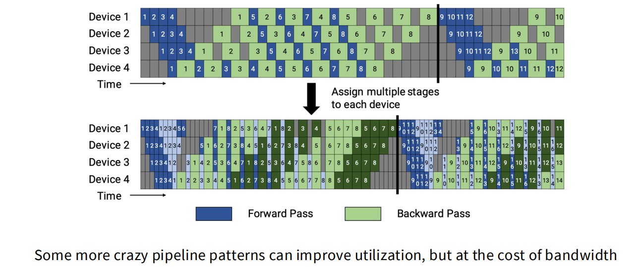
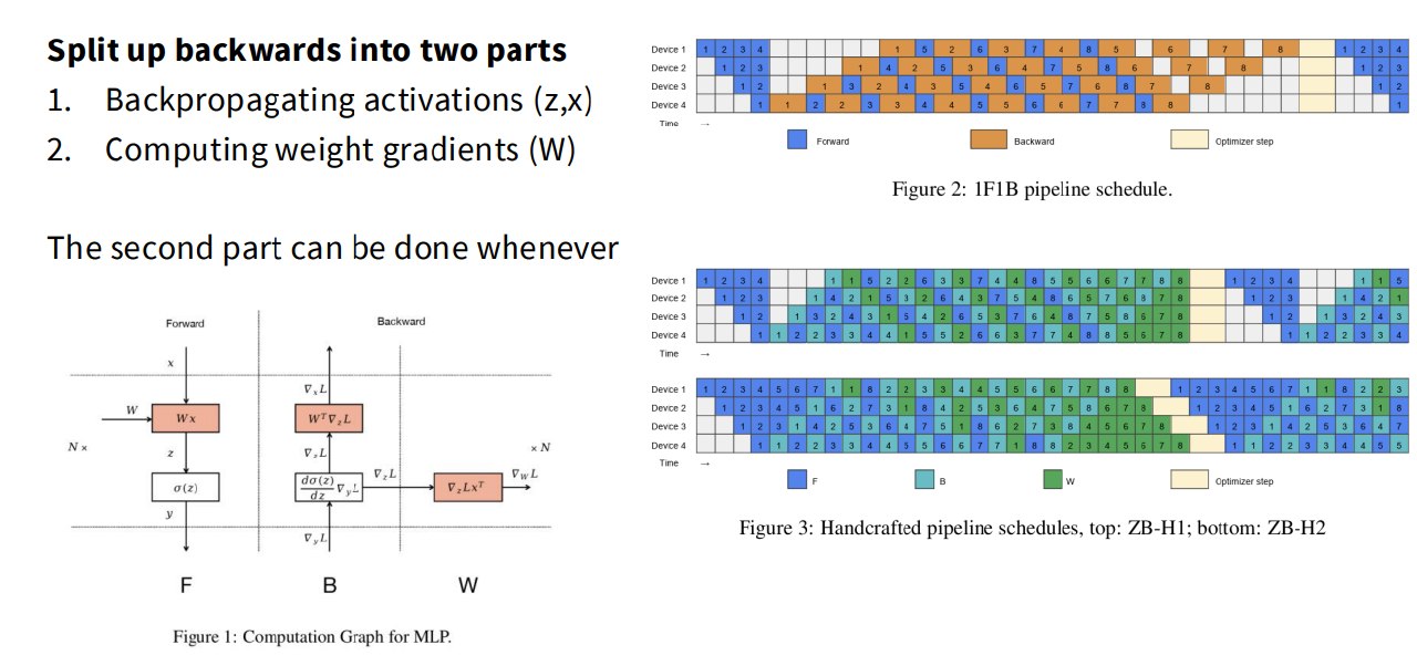
更复杂的 pipeline pattern,包括 zero-bubble pipelining。
Zero-bubble 的关键观察:
Backward 可以拆成两部分:
- activation gradient backpropagation,影响前一层继续反传。
- weight gradient computation,可以更灵活地安排。
如果把 weight gradient computation 塞进原本 bubble 的时间里,就能提高利用率。
2.3.2 Tensor Parallelism:沿 width 切分
Pipeline 是沿 depth 切模型,tensor parallel 是沿 width 切矩阵。
2.3.2.1 矩阵乘法分块
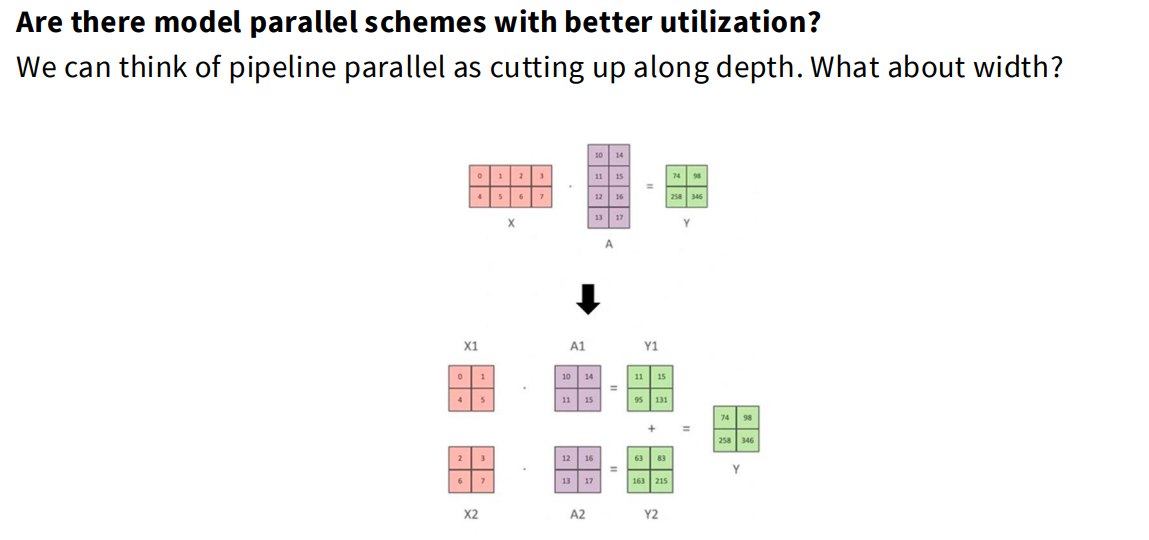
设线性层:
$$ Y = XW $$其中:
$$ X \in \mathbb{R}^{b \times h}, \quad W \in \mathbb{R}^{h \times 4h} $$Column parallel 把 \(W\) 按列切:
$$ W = [W_1, W_2, \dots, W_M] $$每个 rank 计算:
$$ Y_r = XW_r $$最后可以 concat:
$$ Y = [Y_1, Y_2, \dots, Y_M] $$Row parallel 把 \(W\) 按行切:
$$ W = \begin{bmatrix} W_1 \\ W_2 \\ \vdots \\ W_M \end{bmatrix} $$输入 \(X\) 也按 hidden dimension 切成 \(X_r\),每个 rank 计算部分和:
$$ Y_r = X_r W_r $$最后 all-reduce:
$$ Y = \sum_{r=1}^{M} Y_r $$2.3.2.2 Tensor parallel 在 Transformer block 中怎么切
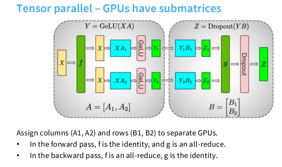
| 模块 | 常见切法 |
|---|---|
| QKV projection | columnwise |
| MLP up-projection | columnwise |
| attention output projection | rowwise |
| MLP down-projection | rowwise |
| LayerNorm / router 等 | replicated |
这种搭配的目的是减少中间通信。例如 MLP 的 up projection 后接 GeLU,再接 down projection,可以让中间 expanded activation 保持 sharded,直到 row-parallel down projection 用 all-reduce 汇总。
伪代码:
# Column-parallel linear.
y_shard = x @ w_col_shard

# Elementwise activation can stay sharded.
y_shard = gelu(y_shard)

# Row-parallel linear produces partial sums.
out_partial = y_shard @ w_row_shard
out = all_reduce_sum(out_partial)
2.3.2.3 什么时候用 tensor parallel
GPU 上通常在单节点内使用 tensor parallel,最多到 8 GPUs 左右,因为它需要高速互联。
对比 pipeline:
Tensor parallel 优点:
- 没有 pipeline bubble。
- 不需要很大 batch size 才有效。
- 模型包装相对直接。
Tensor parallel 缺点:
- 通信量比 pipeline 大。
- 每个 block 都有 activation-sized collectives。
- 强依赖低延迟、高带宽互联。
这个很好理解,pipeline 是层间通信,而tensor 是更细粒度的通信
通信量直觉:
Pipeline 每个 micro-batch 的 point-to-point activation traffic:
$$ O(bsh) $$Tensor parallel 每层 all-reduce activation traffic 约:
$$ O\left(8bsh \cdot \frac{n_{\text{devices}}-1}{n_{\text{devices}}}\right) $$不要死记常数 8,重点是:tensor parallel 的通信发生得更频繁,通常在每个 Transformer block 内。
2.3.3 Activation Memory 与 Sequence Parallelism
前面多在讨论 parameter memory,但训练还要保存 activations。对于长序列,activation memory 可能非常大。
2.3.3.1 Activation memory 为什么动态
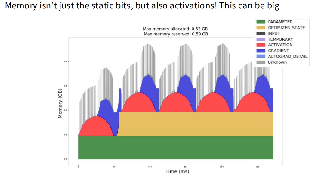
参数显存大致固定,而 activation 显存取决于:
- batch size \(b\)
- sequence length \(s\)
- hidden size \(h\)
- layers
- 是否保存 attention probabilities/dropout mask
- 是否 activation recomputation
一个直观写法:
$$ \text{activation memory per layer} = O(bsh) + O(bs^2) $$其中 $O(bs^2)$ 来自 attention scores/probabilities 等二次项。FlashAttention 或 recomputation 可以避免显式保存很多 $s^2$ 项。
2.3.3.2 Tensor parallel 不能切掉所有 activation
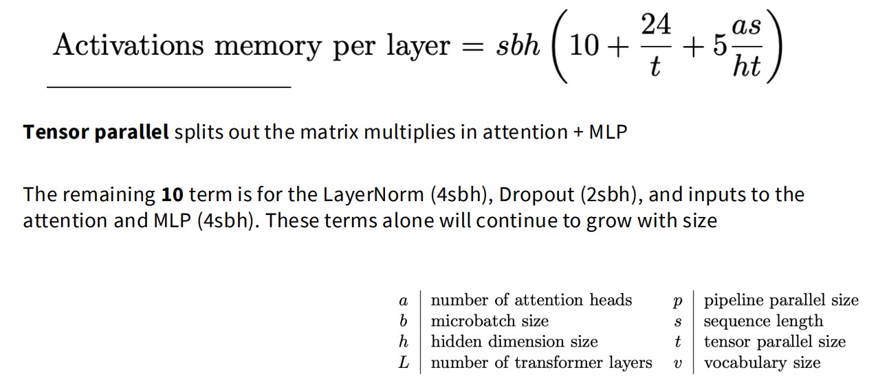
Tensor parallel 可以切分 attention 和 MLP 中的矩阵乘法激活,但 LayerNorm、Dropout、residual 输入等 pointwise operations 仍可能需要完整 sequence-side activation。
剩余的 $10sbh$ 项,包括 LayerNorm、Dropout、attention/MLP 输入等。这些会随模型规模和序列长度继续增长。
2.3.3.3 Sequence Parallel
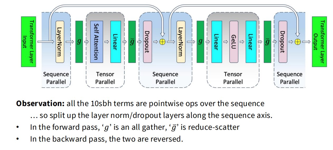
LayerNorm/dropout 等 pointwise ops over sequence,可以沿 sequence axis 切分。
也就是说,把 activation 沿 \(s\) 维切:
$$ X \in \mathbb{R}^{b \times s \times h} $$每个 rank 持有:
$$ X_r \in \mathbb{R}^{b \times (s/M) \times h} $$Forward 中可能需要:
all_gather:在需要完整 hidden/tensor-parallel 布局时收集。reduce_scatter:在 pointwise sequence-sharded 布局中重新分片。
Backward 中通信方向反过来。
伪代码:
# Tensor-parallel region may need hidden-wise shards.
x_tp = all_gather_sequence_shards(x_seq_shard)

# After matmul/attention region, go back to sequence-sharded layout.
x_seq_shard = reduce_scatter_sequence(x_tp)

# Pointwise ops can run independently on sequence shards.
x_seq_shard = layer_norm(x_seq_shard)
x_seq_shard = dropout(x_seq_shard)
Sequence parallel 的目标是让 activation memory 也随机器数线性下降。
2.3.3.4 Context Parallel / Ring Attention
context parallel / ring attention也是沿长序列切 activation/KV,特别适合 long-context training。
直觉:
- Sequence parallel 更强调 Transformer block 内 pointwise activations 的切分。
- Context parallel / ring attention 更强调 attention 中长上下文 KV 的切分和环形通信。
当 s 非常长时,CP 可以显著降低每 rank 的 KV 和 attention memory。
2.4 Expert Parallelism:MoE 的并行方式
MoE 不把一个 dense MLP 的矩阵切成多个 submatrices,而是有多个 experts,每个 token 被 router 分配到部分 experts。
2.4.1 MoE 基本形式
对 token representation \(x\),router 输出 expert 权重:
$$ p(e \mid x) = \mathrm{softmax}(W_r x) $$Top-k routing 选择若干 experts:
$$ \mathcal{E}(x) = \mathrm{TopK}(p(e \mid x)) $$输出可以写成:
$$ y = \sum_{e \in \mathcal{E}(x)} p(e \mid x) f_e(x) $$其中 $f_e$ 是 expert MLP。
2.4.2 Expert parallelism 的通信
Expert parallel 把 experts 分布到不同 ranks。每个 rank 起初持有一批 tokens,但这些 tokens 可能要去其他 ranks 上的 experts。
所以需要 all-to-all:
# tokens: local tokens on each rank
expert_ids = router(tokens)

# Group tokens by destination expert rank.
send_buffers = pack_by_expert_rank(tokens, expert_ids)

# Dispatch tokens to expert owners.
recv_buffers = all_to_all(send_buffers)

# Run local experts.
expert_outputs = run_local_experts(recv_buffers)

# Send outputs back to original token owners.
outputs = all_to_all(expert_outputs)
2.4.3 为什么用 EP(Expert Parallelism)
EP 对 MLP 的行为有点像 TP:
- 都能降低每 rank 的参数和计算负担。
- 都需要高带宽通信。
但 EP 的优势是:不拆 dense matmul,而是把 token 路由到完整 expert。拆 matmul 可能降低 GEMM efficiency;MoE 如果 routing 和 load balance 做得好,可以让每个 expert 做较大的局部 matmul。
2.4.4 EP 的复杂性
- EP 可以和 DP/TP/PP 组合。
- DP 通常和 EP split 共享 replica 结构。
- DP 和 TP 组合不当可能降低利用率。
- MoE 主要作用于 MLP,不作用于 attention。
因此 attention 和 MLP 的最佳并行策略可能不同:
- Attention 可能需要较高 TP 或 CP。
- MLP 更想用 EP。
Megatron-Core 中会更细地区分:
- attention 侧:TP/CP/DP
- MoE MLP 侧:ETP/EP/EDP
这就是为什么真实大模型训练配置看起来像一串并行维度,而不是单个开关。
2.5 LLM Parallelism 总表
| 方法 | 通信/同步 | 每 rank 参数显存 | 激活/KV 显存 | 主要带宽成本 | 是否扩展 global batch | 易用性 |
|---|---|---|---|---|---|---|
| DDP / ZeRO-1 | 每 step gradient all-reduce | 参数不缩放,ZeRO-1 只切 optimizer state | 不缩放 | gradient traffic \(O(\text{params})\) | 是 | 容易 |
| FSDP / ZeRO-3 | 参数 all-gather + 梯度 reduce-scatter,可 overlap | 约 \(1/\text{DP}\) | 不直接缩放 | parameter traffic,通常高于 DDP | 是 | 中等 |
| Pipeline parallel | stage 间 activation,存在 bubble | 约 \(1/\text{PP}\) | 取决于 buffers | stage 间 activation traffic | 否,但需要 microbatches | 难 |
| Tensor parallel | 每 block activation collectives | TP-sharded weights 约 \(1/\text{TP}\) | 相关 matmul activations 可缩放,配合 SP 更好 | activation-sized collectives | 否 | 难 |
| Sequence / Context parallel | sequence-shard exchange | 不缩放参数 | sequence/KV 侧约 \(1/\text{SP/CP}\) | activation/KV communication | 否 | 难 |
| Expert parallel | MoE token dispatch all-to-all | expert weights 约 \(1/\text{EP}\) | 通常不直接缩放 | token-routing all-to-all | 否,但需要足够 tokens/expert | 难 |
这张表的重点是:没有单一方法解决所有瓶颈。我们通常要组合它们。
三、3D/4D Parallelism
主要是讲如何组合并行策略。
3.1 经验规则
讲义给出简单 rules of thumb:
- 在模型还不能 fit 之前:
- 节点内优先用 tensor/expert parallel。
- 跨机器用 pipeline parallel。
- 或者根据带宽条件用 ZeRO-3。
- 当模型能 fit 后:
- 剩余 GPU 用 data parallel 扩展吞吐。
- 如果 batch size 小:
- 用 gradient accumulation 增大 effective batch,提高通信效率。
Effective batch 可以写为:
$$ B_{\text{effective}} = B_{\text{micro}} \times n_{\text{micro}} \times \text{DP} $$如果有 gradient accumulation steps \(G\):
$$ B_{\text{effective}} = B_{\text{micro}} \times n_{\text{micro}} \times G \times \text{DP} $$3.2 TP 通常先到 8
讲义引用 Narayanan 2021 之类的 scaling strategy:TP 先增加到 8,然后 caps out。
原因:
- 单节点通常 8 GPUs,NVLink/NVSwitch 快。
- TP 跨节点通信太频繁,收益会下降。
所以常见结构:
TP = GPUs per node, e.g. 8
PP = number of model stage groups across nodes
DP = remaining replicas
3.3 Activation recomputation 的价值
activation recomputation can pay for itself。
Activation recomputation / checkpointing 的思想:
- forward 时不保存所有中间 activations。
- backward 时重新计算一部分 activations。
- 用额外 compute 换显存。
如果省下的显存允许更大的 batch 或更优的 parallelism 配置,整体 throughput 可能更高。
四、系统瓶颈总结
本讲不是在列并行名词,而是在建立系统判断力。
4.1 显存瓶颈
显存由多类组成:
$$ \text{memory} = \text{params}
- \text{grads}
- \text{optimizer states}
- \text{activations}
- \text{temporary buffers}
- \text{KV/cache} $$
ZeRO/FSDP 主要解决 params/grads/optimizer states。Sequence/context parallel 和 activation recomputation 解决 activation/KV。
4.2 通信带宽瓶颈
不同策略通信对象不同:
- DDP:gradients。
- FSDP:parameters + gradients。
- Pipeline:activations between stages。
- Tensor:activation collectives every block。
- EP:token dispatch all-to-all。
- CP:KV/sequence shards。
选择并行策略时,要问:
这个通信发生多频繁?跨不跨节点?能否 overlap?
4.3 Pipeline bubble
Pipeline 的主要问题是 bubble:
$$ \text{bubble ratio} \approx \frac{n_{\text{stages}} - 1}{n_{\text{micro}}} $$解决方式:
- 增加 micro-batches。
- 使用 1F1B schedule。
- interleaving。
- zero-bubble pipeline。
代价是调度复杂度和可能更高通信/内存需求。
4.4 MoE load balancing
Expert parallel 的核心风险是 token 分配不均。若某些 experts 收到太多 tokens,它们会成为 straggler。
常见缓解:
- router auxiliary load-balancing loss。
- capacity factor。
- token dropping 或 padding。
- all-to-all overlap。
MoE 的系统问题往往比数学公式更棘手。
4.5 可靠性
Llama 3 405B 这类规模会遇到大量 GPU failures。GPU 数越多,任意时刻发生故障的概率越高。
大规模训练需要:
- checkpointing。
- elastic restart。
- failure detection。
- deterministic replay 或可接受的非确定恢复。
- 数据加载和随机种子的恢复。
这也是“训练大模型”成为系统工程的原因。

说些什么吧!