多GPU并行训练

2026-06-16

零、写在前面

lecture07 主要就是介绍了一些分布式GPU训练策略。

一、多 GPU 并行训练

1.1 为什么需要多 GPU

之前讲的 warps、thread blocks、shared memory、tiling、fusion，这些都是 单 GPU 内部并行。核心问题是：计算单元离数据很远，要减少 HBM 访问。

本讲扩展到 多 GPU/多节点并行。核心问题变成：计算在多张 GPU 上，数据、参数、梯度和激活也分散在多张 GPU 上，要减少 GPU 之间、节点之间的数据传输。

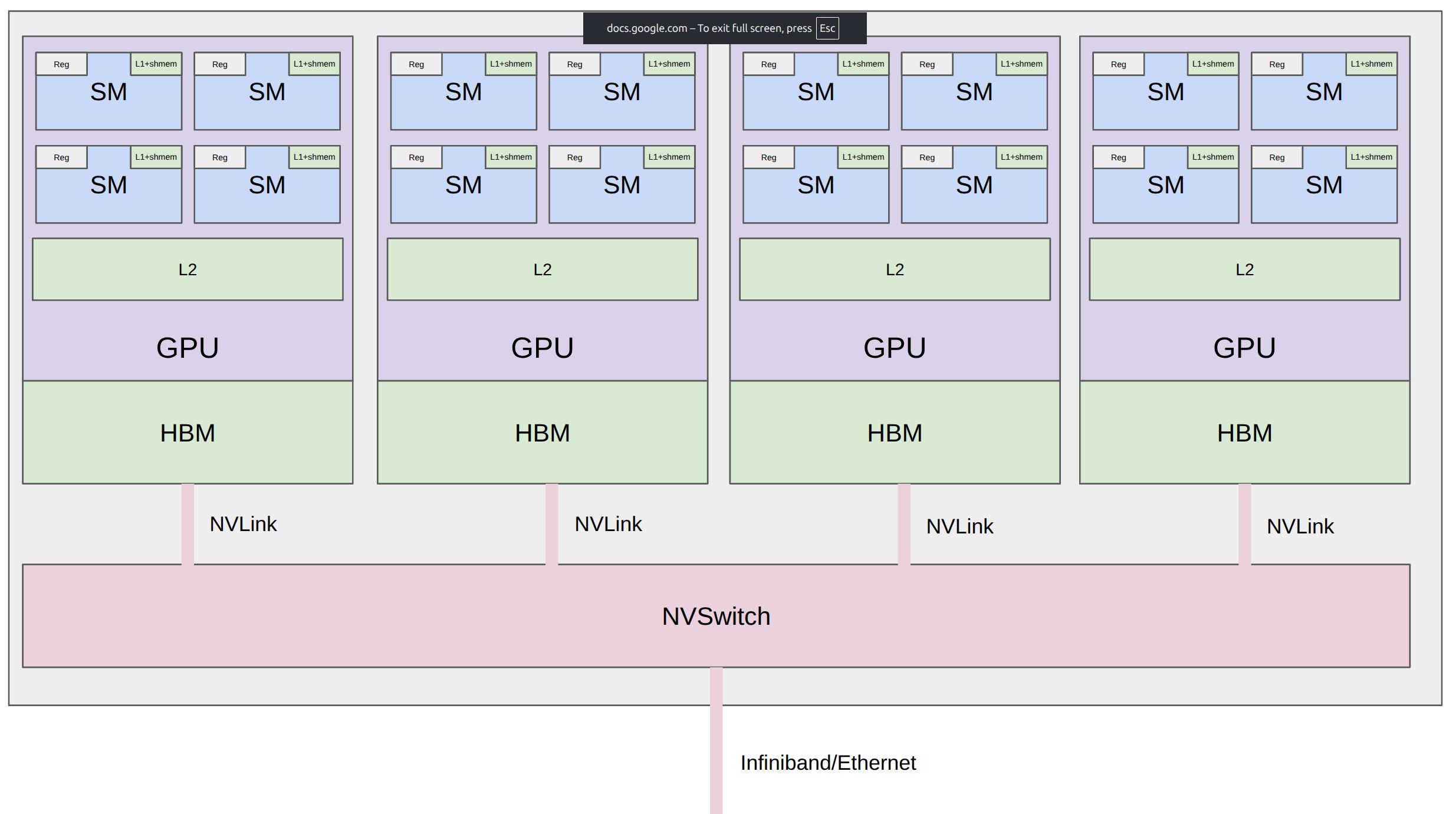
一个粗略的通信层次是：

层次	例子	速度直觉
单 GPU 内部	registers / shared memory / L1	最快
单 GPU 显存	HBM	很快，但比片上存储慢
单节点多 GPU	NVLink / NVSwitch / PCIe	比 HBM 慢
多节点	InfiniBand / Ethernet	最慢

因此本讲的统一主题是：

orchestrate computation to avoid data transfer bottlenecks

为什么要多 GPU？

放不下：参数、optimizer state、梯度、激活可能超过单卡显存。
想更快：使用更多 GPU FLOPs，提高训练吞吐。

但增加 GPU 不会自动变快。只要通信成为瓶颈，更多 GPU 可能只是在更快地等待彼此。

1.2 Collective Operations：分布式通信原语

多 GPU 编程中，不直接手写每一对 GPU 的 send/recv，通常使用 collective operations。Collective 表示所有 ranks 共同参与某种通信模式。

基本术语：

rank：某个进程/设备的编号，例如 0, 1, 2, 3。
world size：参与通信的 rank 总数，例如 4。
process group：参与某组 collective 的进程集合；本讲默认所有 ranks 在同一个 group 里。

1.2.1 Broadcast

Broadcast 是从一个源 rank 复制到所有 ranks。

输入：

rank0 = tensor([0., 1, 2, 3])

输出：

rank0 = tensor([0., 1, 2, 3])
rank1 = tensor([0., 1, 2, 3])
rank2 = tensor([0., 1, 2, 3])
rank3 = tensor([0., 1, 2, 3])

典型场景：rank 0 读取 checkpoint，然后广播初始参数到所有 ranks。

1.2.2 Scatter 与 Gather

Scatter 把 rank 0 上的 tensor 拆开，发给各个 ranks。

# input on rank 0
rank0 = tensor([0., 1, 2, 3])

# output
rank0 = tensor([0.])
rank1 = tensor([1.])
rank2 = tensor([2.])
rank3 = tensor([3.])

Gather 是反方向：各 rank 的 pieces 聚合到 rank 0。

# input
rank0 = tensor([0.])
rank1 = tensor([1.])
rank2 = tensor([2.])
rank3 = tensor([3.])

# output on rank 0
rank0 = tensor([0., 1, 2, 3])

这两个操作本身不一定是训练最常用的，但它们是理解 all_gather 和 reduce_scatter 的台阶。

1.2.3 Reduce

Reduce 从所有 ranks 收集值，并做一个 associative/commutative operation，例如 sum、min、max。

# input
rank0 = tensor([0.])
rank1 = tensor([1.])
rank2 = tensor([2.])
rank3 = tensor([3.])

# sum output on rank 0
rank0 = tensor([6.])

训练里最常见的是 sum 或 average gradients。

1.2.4 All-gather

All-gather 是 gather 到所有 ranks，而不只是 rank 0。

# input
rank0 = tensor([0.])
rank1 = tensor([1.])
rank2 = tensor([2.])
rank3 = tensor([3.])

# output on every rank
tensor([0., 1, 2, 3])

用例：每个 rank 持有参数 shard，forward 前 all-gather 得到完整参数。

1.2.5 Reduce-scatter

Reduce-scatter 可以理解为：

先沿 rank 维度 reduce。
再把 reduce 后的结果 scatter 到不同 ranks。

输入：

rank0 = tensor([0., 1, 2, 3])
rank1 = tensor([1., 2, 3, 4])
rank2 = tensor([2., 3, 4, 5])
rank3 = tensor([3., 4, 5, 6])

输出：

rank0 = tensor([6.])   # 0 + 1 + 2 + 3
rank1 = tensor([10.])  # 1 + 2 + 3 + 4
rank2 = tensor([14.])  # 2 + 3 + 4 + 5
rank3 = tensor([18.])  # 3 + 4 + 5 + 6

用例：backward 后不同 data shards 产生梯度，把梯度求和后分片存储。这是 ZeRO/FSDP 背后的核心通信之一。

1.2.6 All-reduce

All-reduce 是最常见的训练 collective。它可以看成：

all-reduce = reduce-scatter + all-gather

输入：

rank0 = tensor([0., 1, 2, 3])
rank1 = tensor([1., 2, 3, 4])
rank2 = tensor([2., 3, 4, 5])
rank3 = tensor([3., 4, 5, 6])

输出到每个 rank：

tensor([6., 10, 14, 18])

数据并行里，每个 rank 计算本地梯度 ($g_r$)，然后平均：

$$ g = \frac{1}{P}\sum_{r=0}^{P-1} g_r $$

其中 $P$ 是 world size。PyTorch 里可以用 ReduceOp.AVG 直接平均，也可以用 sum 后除以 $P$。

1.2.7 All-to-all

All-to-all 是更一般的通信：每个 rank 给每个其他 rank 发一块数据。

rank0 = tensor([0., 1, 2, 3])      # send to ranks 0,1,2,3
rank1 = tensor([4., 5, 6, 7])
rank2 = tensor([8., 9, 10, 11])
rank3 = tensor([12., 13, 14, 15])

输出：

rank0 = tensor([0, 4, 8, 12])
rank1 = tensor([1, 5, 9, 13])
rank2 = tensor([2, 6, 10, 14])
rank3 = tensor([3, 7, 11, 15])

MoE 中常见 all-to-all：token 根据 router 被分发到不同 expert 所在的 rank。balanced split 时，它看起来像 transpose；不均衡时还要处理 variable splits。

总结就是：

reduce：做 sum/min/max 等归约。
scatter 是 gather 的反方向。
all 表示目的地是所有 ranks。

1.3 硬件互联与 NCCL

多 GPU 性能高度依赖互联拓扑。

1.3.1 从家用机器到数据中心

经典家用机器里，GPU 往往通过 PCIe 连接。不同节点之间可能通过普通 Ethernet 通信，延迟更高、带宽更低。

数据中心训练集群通常更复杂：

典型形态：

单节点：8 GPUs，通过 NVLink 连接到 NVSwitch。
多节点：节点之间通过 InfiniBand 或 RoCE 互联。
更大集群：多个 pod / rack 之间再通过更慢的网络层连接。

讲义给出的直觉数字：

B200 NVLink 5.0 约 1.8 TB/s。
B200 HBM 约 8 TB/s。
InfiniBand 约 0.05 TB/s。

数值不重要，关键是比例：跨 GPU 比单 GPU HBM 慢，跨节点又比单节点互联慢。

1.3.2 RDMA 与绕过 CPU

普通 Ethernet 通常要经过 CPU 和内核网络栈：

GPU/CPU memory -> kernel socket buffer -> TCP packet -> NIC ring buffer -> network

RDMA 允许一台机器直接读写另一台机器的内存，减少 CPU 参与。InfiniBand 支持 RDMA；RoCE 是在以太网上实现类似 RDMA 的方案。

训练系统里，能绕开 CPU 就少一次瓶颈。

1.3.3 NCCL 的角色

NCCL 是 NVIDIA Collective Communication Library。它负责把 all_reduce、all_gather 等 collective operations 翻译成 GPU 间的高效通信。

NCCL 做的事包括：

检测拓扑：GPU 数量、NVLink、PCIe、交换机、节点间连接。
为 collective 选择通信路径和算法。
启动 GPU kernels 来搬运和规约数据。

在 PyTorch 中，GPU collective 通常通过 backend="nccl" 使用 NCCL。CPU collective 常用 backend="gloo"。

1.4 PyTorch Distributed

讲义提供了 pytroch distributed 的代码示例

1.4.1 分布式入口

def setup(rank: int, world_size: int):
    os.environ["MASTER_ADDR"] = "localhost"
    os.environ["MASTER_PORT"] = "15623"

    if torch.cuda.is_available():
        dist.init_process_group("nccl", rank=rank, world_size=world_size)
    else:
        dist.init_process_group("gloo", rank=rank, world_size=world_size)

MASTER_ADDR 和 MASTER_PORT 用于进程发现和协调。
rank 0 作为 rendezvous 的中心。
有 CUDA 时使用 NCCL；否则使用 Gloo。

process group 清理：

def cleanup():
    torch.distributed.destroy_process_group()

1.4.2 spawn：启动多个ranks

讲义用 spawn() 封装多进程：

import torch.multiprocessing as mp

def spawn(func: Callable, world_size: int, *args, **kwargs):
    if not sys.gettrace():
        args = (world_size,) + args + tuple(kwargs.values())
        mp.spawn(func, args=args, nprocs=world_size, join=True)
    else:
        with DisableDistributed():
            args = (0, world_size,) + args + tuple(kwargs.values())
            func(*args)

普通执行时：

mp.spawn 启动 world_size 个进程。
每个进程调用同一个函数。
函数第一个参数是 rank，第二个参数是 world_size。

edtrace trace 时：

不真正启动多进程。
用 DisableDistributed 把 torch.distributed 函数替换成 no-op。
这样可以生成讲义 trace，但不能代表真实通信。

1.4.3 all-reduce、reduce-scatter、all-gather

import torch.distributed as dist

def collective_operations_main(rank: int, world_size: int):  # @inspect rank world_size
    """This function is running asynchronously for each process (rank = 0, ..., world_size - 1)."""
    setup(rank, world_size)

    ### All-reduce (dist = torch.distributed)
    dist.barrier()  # Waits for all processes to get to this point (in this case, for print statements)

    data = tensor([0., 1, 2, 3], device=cuda_if_available(rank)) + rank  # Both input and output

    print(f"Rank {rank} [before all-reduce]: {data}", flush=True)
    dist.all_reduce(tensor=data, op=dist.ReduceOp.SUM, async_op=False)  # Modifies tensor in place
    print(f"Rank {rank} [after all-reduce]: {data}", flush=True)

    ### Reduce-scatter
    dist.barrier()

    input = torch.arange(world_size, dtype=torch.float32, device=cuda_if_available(rank)) + rank  # Input
    output = torch.empty(1, device=cuda_if_available(rank))  # Allocate output

    print(f"Rank {rank} [before reduce-scatter]: input = {input}, output = {output}", flush=True)
    dist.reduce_scatter_tensor(output=output, input=input, op=dist.ReduceOp.SUM, async_op=False)
    print(f"Rank {rank} [after reduce-scatter]: input = {input}, output = {output}", flush=True)

    ### All-gather
    dist.barrier()

    input = output  # Input is the output of reduce-scatter
    output = torch.empty(world_size, device=cuda_if_available(rank))  # Allocate output

    print(f"Rank {rank} [before all-gather]: input = {input}, output = {output}", flush=True)
    dist.all_gather_into_tensor(output_tensor=output, input_tensor=input, async_op=False)
    print(f"Rank {rank} [after all-gather]: input = {input}, output = {output}", flush=True)

    text("Indeed, all-reduce = reduce-scatter + all-gather!")

    cleanup()

第一段 all-reduce：

data = tensor([0., 1, 2, 3], device=cuda_if_available(rank)) + rank

dist.all_reduce(tensor=data, op=dist.ReduceOp.SUM, async_op=False)

每个 rank 初始数据不同：

rank 0: [0, 1, 2, 3]
rank 1: [1, 2, 3, 4]
rank 2: [2, 3, 4, 5]
rank 3: [3, 4, 5, 6]

all-reduce sum 后，每个 rank 都得到：

[6, 10, 14, 18]

第二段 reduce-scatter：

input = torch.arange(world_size, dtype=torch.float32, device=cuda_if_available(rank)) + rank
output = torch.empty(1, device=cuda_if_available(rank))

dist.reduce_scatter_tensor(output=output, input=input, op=dist.ReduceOp.SUM)

每个 rank 的输入长度是 world_size，输出长度是 1。reduce-scatter 后，每个 rank 只保留归约结果的一片。

第三段 all-gather：

input = output
output = torch.empty(world_size, device=cuda_if_available(rank))

dist.all_gather_into_tensor(output_tensor=output, input_tensor=input)

这一步把 reduce-scatter 后的 shards 再收集到每个 rank，于是恢复成 all-reduce 的完整输出。这就是原讲义强调的：

all-reduce = reduce-scatter + all-gather

1.5 通信Benchmark

训练吞吐不是只看 FLOPs，还要看 communication。原讲义 benchmark 了 all_reduce 和 reduce_scatter。

1.5.1 all_reduce benchmark

先 warmup，避免第一次初始化影响计时。
torch.cuda.synchronize() 等待 GPU kernel 完成。
dist.barrier() 等待所有 ranks 到达同一点。
只测第二次 collective 的耗时。

def all_reduce(rank: int, world_size: int, num_elements: int):
    setup(rank, world_size)  # @stepover

    # Create tensor
    data = torch.randn(num_elements, device=cuda_if_available(rank))

    # Warmup
    dist.all_reduce(tensor=data, op=dist.ReduceOp.SUM, async_op=False)
    torch.cuda.synchronize()  # Wait for CUDA kernels to finish
    dist.barrier()            # Wait for all the processes to get here

    # Perform all-reduce
    start_time = time.time()
    dist.all_reduce(tensor=data, op=dist.ReduceOp.SUM, async_op=False)
    torch.cuda.synchronize()  # Wait for CUDA kernels to finish
    dist.barrier()            # Wait for all the processes to get here
    end_time = time.time()

    duration = end_time - start_time
    print(f"[all_reduce] Rank {rank}: all_reduce(world_size={world_size}, num_elements={num_elements}) took {render_duration(duration)}", flush=True)  # @stepover

    # Measure the effective bandwidth
    dist.barrier()
    size_bytes = data.element_size() * data.numel()
    sent_bytes = size_bytes * 2 * (world_size - 1)  # 2x because send + receive, world_size-1 steps in all-reduce
    total_duration = world_size * duration
    bandwidth = sent_bytes / total_duration
    print(f"[all_reduce] Rank {rank}: all_reduce measured bandwidth = {round(bandwidth / 1024**3)} GB/s", flush=True)

    # Notes:
    # - Effective bandwidth ~ 2 * size_bytes / total_duration
    # - Independent of world_size
    # - Independent of topology (ring or tree)

    cleanup()  # @stepover

有效带宽估计：

size_bytes = data.element_size() * data.numel()
sent_bytes = size_bytes * 2 * (world_size - 1)
total_duration = world_size * duration
bandwidth = sent_bytes / total_duration

直觉解释：

Ring all-reduce 可以拆成 reduce-scatter 和 all-gather 两个阶段。所以sent_bytes 要乘2
每个阶段大致要经过 $P-1$ 步。因为要做 rank0 + rank1 + …
所以代码用 $2(P-1)$ 估计 send/receive 数据量。

如果单个 rank 上 tensor 大小是 $S$ bytes，world size 是 $P$，代码中的近似通信量是：

$$ \text{sent\_bytes} \approx 2S(P-1) $$

代码又把 duration 乘以 world_size 得到 total_duration，最后输出一个粗略 measured bandwidth。这个数适合做同一环境下的相对比较，不要当作硬件理论峰值。

1.5.2 reduce_scatter benchmark

def reduce_scatter(rank: int, world_size: int, num_elements: int):
    setup(rank, world_size)  # @stepover

    # Create input and outputs
    input = torch.randn(world_size, num_elements, device=cuda_if_available(rank))  # Each rank has a matrix
    output = torch.empty(num_elements, device=cuda_if_available(rank))

    # Warmup
    dist.reduce_scatter_tensor(output=output, input=input, op=dist.ReduceOp.SUM, async_op=False)
    torch.cuda.synchronize()  # Wait for CUDA kernels to finish
    dist.barrier()            # Wait for all the processes to get here

    # Perform reduce-scatter
    start_time = time.time()
    dist.reduce_scatter_tensor(output=output, input=input, op=dist.ReduceOp.SUM, async_op=False)
    torch.cuda.synchronize()  # Wait for CUDA kernels to finish
    dist.barrier()            # Wait for all the processes to get here
    end_time = time.time()

    duration = end_time - start_time
    print(f"[reduce_scatter] Rank {rank}: reduce_scatter(world_size={world_size}, num_elements={num_elements}) took {render_duration(duration)}", flush=True)  # @stepover

    # Measure the effective bandwidth
    dist.barrier()
    data_bytes = input.element_size() * input.numel()  # How much data in the input
    sent_bytes = data_bytes * (world_size - 1)  # How much needs to be sent (no 2x here)
    total_duration = world_size * duration  # Total time for transmission
    bandwidth = sent_bytes / total_duration
    print(f"[reduce_scatter] Rank {rank}: reduce_scatter measured bandwidth = {round(bandwidth / 1024**3)} GB/s", flush=True)

    # Notes:
    # - all-reduce = reduce-scatter + all-gather
    # - all-reduce moves 2x the data in 2x the time compared to reduce-scatter, so similar bandwidth

    cleanup()  # @stepover

input = torch.randn(world_size, num_elements, device=cuda_if_available(rank))
output = torch.empty(num_elements, device=cuda_if_available(rank))

dist.reduce_scatter_tensor(output=output, input=input, op=dist.ReduceOp.SUM)

这里每个 rank 的 input 是一个矩阵：

[world_size, num_elements]

reduce-scatter 后，每个 rank 只得到一段 output：

[num_elements]

带宽估计：

data_bytes = input.element_size() * input.numel()
sent_bytes = data_bytes * (world_size - 1)
total_duration = world_size * duration
bandwidth = sent_bytes / total_duration

1.6 Distributed Training：三种并行策略

原讲义用 deep MLP 做最小训练系统。原因是 Transformer 中 MLP 通常是主要 compute bottleneck 之一，用 MLP 可以看清并行策略，而不被 attention 细节干扰。

统一的单层 MLP 计算是：

$$ X_{\ell+1} = \mathrm{GeLU}(X_\ell W_\ell) $$

其中：

$X_\ell \in \mathbb{R}^{B \times D}$
$W_\ell \in \mathbb{R}^{D \times D}$
$ B 是 batch size$
$D 是 hidden \ dimension$

并行训练的核心问题是：沿哪个维度切？

并行策略	切分维度	每个 rank 持有什么	主要通信
Data parallelism	batch	完整模型 + 一份数据	gradients all-reduce
Tensor parallelism	width / hidden dim	每层参数的一片	activations all-gather / reduce
Pipeline parallelism	depth / layers	连续几层	stage 间 send/recv activations

1.7 Data Parallelism：沿 batch 维切数据

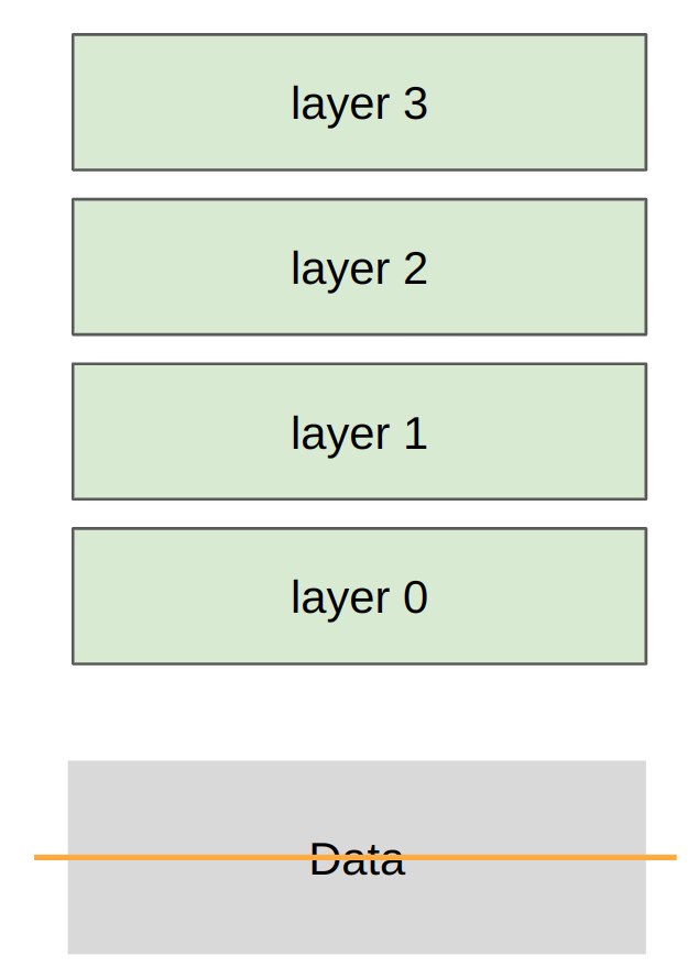
Data parallelism 的 sharding strategy：

each rank gets a slice of the data

每个 rank 拿完整模型参数，但只处理 batch 的一部分。

如果有 P 个 ranks，每个 rank 的 local batch 是 $B_{\text{local}}$，那么：

$$ B_{\text{global}} = P \cdot B_{\text{local}} $$

测试函数

def data_parallelism_main(rank: int, world_size: int, data: tensor, num_layers: int, num_steps: int):
    setup(rank, world_size)  # @stepover

    # Get the slice of data for this rank (in practice, each rank should load only its own data)
    # --- B0 ---
    # --- B1 ---
    # --- B2 ---
    # --- B3 ---
    batch_size = data.size(0)  # @inspect batch_size
    num_dim = data.size(1)  # @inspect num_dim
    local_batch_size = int_divide(batch_size, world_size)  # @inspect local_batch_size @stepover
    start_index = rank * local_batch_size  # @inspect start_index
    end_index = start_index + local_batch_size  # @inspect end_index
    data = data[start_index:end_index].to(cuda_if_available(rank))

    # Create MLP parameters params[0], ..., params[num_layers - 1] (each rank has all parameters)
    params = [get_init_params(num_dim, num_dim, rank) for layer in range(num_layers)]
    optimizer = torch.optim.AdamW(params, lr=1e-3)  # Each rank has own optimizer state

    for step in range(num_steps):
        # Forward pass
        x = data
        for param in params:
            x = x @ param
            x = F.gelu(x)
        loss = x.square().mean()  # Loss function is average squared magnitude

        # Backward pass
        loss.backward()

        # Sync gradients across workers (ONLY difference between standard training and DDP)
        for param in params:
            dist.all_reduce(tensor=param.grad, op=dist.ReduceOp.AVG, async_op=False)

        # Update parameters
        optimizer.step()

        print(f"[data_parallelism] Rank {rank}: step = {step}, loss = {loss.item()}, params = {[summarize_tensor(params[layer]) for layer in range(num_layers)]}", flush=True)  # @stepover

    cleanup()  # @stepover

1.7.1 数据生成

def generate_sample_data():
    batch_size = 128
    num_dim = 1024
    data = torch.randn(batch_size, num_dim)
    return data

这里：

batch size 是 128。
hidden dimension 是 1024。
数据先在 CPU 上生成，后面各 rank 取 slice 并搬到自己的 device。

1.7.2 每个 rank 取自己的 batch slice

batch_size = data.size(0)
num_dim = data.size(1)
local_batch_size = int_divide(batch_size, world_size)
start_index = rank * local_batch_size
end_index = start_index + local_batch_size
data = data[start_index:end_index].to(cuda_if_available(rank))

如果 world_size=4，batch size 128，那么每个 rank 处理 32 条样本。

1.7.3 每个 rank 持有完整参数

params = [get_init_params(num_dim, num_dim, rank) for layer in range(num_layers)]
optimizer = torch.optim.AdamW(params, lr=1e-3)

get_init_params() 中使用相同 seed：

torch.random.manual_seed(0)

所以每个 rank 初始化得到相同参数。每个 rank 还有自己的 AdamW optimizer state。

1.7.4 Forward 与 backward

x = data
for param in params:
    x = x @ param
    x = F.gelu(x)
loss = x.square().mean()

loss.backward()

每个 rank 的 loss 可能不同，因为它看到的数据不同。但模型参数初始相同。

1.7.5 梯度同步

Data parallelism 和普通单卡训练唯一关键差异是：

for param in params:
    dist.all_reduce(tensor=param.grad, op=dist.ReduceOp.AVG, async_op=False)

这一步让所有 ranks 的梯度一致：

$$ g = \frac{1}{P}\sum_{r=0}^{P-1} g_r $$

然后各 rank 执行相同 optimizer step：

optimizer.step()

因为参数初始相同、梯度同步后也相同、optimizer state 的更新也相同，所以参数会保持一致。

原讲义备注：

losses 不同：因为每个 rank 的 local data 不同。
gradients 相同：因为 all-reduce 后同步。
parameters 相同：因为每个 rank 用相同梯度更新相同初始参数。

1.7.6 与 DDP/FSDP 的关系

这个示例是 bare-bones DDP 思想。真实 PyTorch DistributedDataParallel 会自动注册 backward hooks，在梯度产生时分 bucket 做 all-reduce，并尽量 overlap communication and computation。

FSDP/ZeRO 进一步减少显存占用：不让每个 rank 永远持有完整参数、梯度和 optimizer state，而是通过 all-gather 与 reduce-scatter 在需要时重建/分片。

1.8 Tensor Parallelism：沿 width 维切参数

def tensor_parallelism():
    image("images/tensor-parallelism.png", width=300)
    text("Sharding strategy: each rank gets part of each layer, transfer all data/activations")

    data = generate_sample_data()
    spawn(tensor_parallelism_main, world_size=4, data=data, num_layers=4)

def tensor_parallelism_main(rank: int, world_size: int, data: tensor, num_layers: int):
    setup(rank, world_size)  # @stepover

    data = data.to(cuda_if_available(rank))  # All ranks get the data (batch_size x num_dim)
    batch_size = data.size(0)  # @inspect batch_size
    num_dim = data.size(1)  # @inspect num_dim
    local_num_dim = int_divide(num_dim, world_size)  # Shard `num_dim`  @inspect local_num_dim @stepover

    # Create model (each rank gets 1/world_size of the parameters)
    #  |  |  |  |
    # W0 W1 W2 W3
    #  |  |  |  |
    params = [get_init_params(num_dim, local_num_dim, rank) for layer in range(num_layers)]

    # Forward pass
    x = data
    for layer in range(num_layers):
        # Compute activations (batch_size x local_num_dim)
        x = x @ params[layer]  # Note: this is only on a slice of the parameters
        x = F.gelu(x)

        # Allocate memory for activations (world_size x batch_size x local_num_dim)
        activations = [torch.empty(batch_size, local_num_dim, device=cuda_if_available(rank)) for _ in range(world_size)]

        # Send activations via all gather
        dist.all_gather(tensor_list=activations, tensor=x, async_op=False)

        # Concatenate them to get batch_size x num_dim
        x = torch.cat(activations, dim=1)

    print(f"[tensor_parallelism] Rank {rank}: forward pass produced activations {summarize_tensor(x)}", flush=True)  # @stepover

    # Backward pass: homework exercise

    cleanup()  # @stepover

图示：

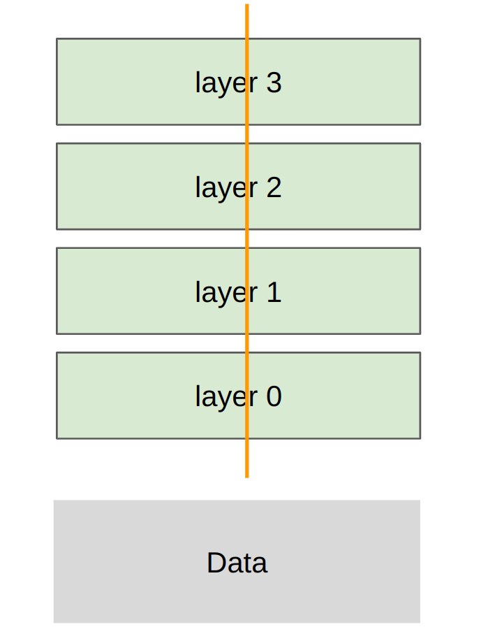
Tensor parallelism 的 sharding strategy：

each rank gets part of each layer, transfer all data/activations

Data parallelism 是每个 rank 有完整层；tensor parallelism 是每层参数被切开。

1.8.1 参数切分

data = data.to(cuda_if_available(rank))
batch_size = data.size(0)
num_dim = data.size(1)
local_num_dim = int_divide(num_dim, world_size)

params = [get_init_params(num_dim, local_num_dim, rank) for layer in range(num_layers)]

每个 rank 持有每层权重的一部分：

$$ W_\ell^{(r)} \in \mathbb{R}^{D \times D/P} $$

如果完整权重是：

$$ W_\ell \in \mathbb{R}^{D \times D} $$

那么按列切分：

$$ W_\ell = [W_\ell^{(0)}, W_\ell^{(1)}, \dots, W_\ell^{(P-1)}] $$

1.8.2 本地 matmul

x = x @ params[layer]
x = F.gelu(x)

输入 $X \in \mathbb{R}^{B \times D}$，本地权重 $W^{(r)} \in \mathbb{R}^{D \times D/P}$，所以本地输出是：

$$ X W^{(r)} \in \mathbb{R}^{B \times D/P} $$

每个 rank 只算输出 hidden dimension 的一片。

1.8.3 All-gather 激活

activations = [
    torch.empty(batch_size, local_num_dim, device=cuda_if_available(rank))
    for _ in range(world_size)
]

dist.all_gather(tensor_list=activations, tensor=x, async_op=False)

x = torch.cat(activations, dim=1)

每个 rank 计算一个 activation shard，然后 all-gather 到所有 ranks，最后拼接回完整 hidden dimension：

$$ X_{\ell+1} = \mathrm{concat}\left( X_{\ell+1}^{(0)}, \dots, X_{\ell+1}^{(P-1)} \right) \in \mathbb{R}^{B \times D} $$

这个版本为了教学简单，每一层都 all-gather 完整 activation。真实 Megatron-LM 风格 tensor parallel 会交替使用 column-parallel 和 row-parallel linear，使通信位置更少、更精细。

1.8.4 为什么 tensor parallelism 需要高速互联

Tensor parallelism 的通信发生在层内或层间，频率很高。每一层都可能要 gather/reduce activations 或 gradients，所以它通常要求很快的 GPU-GPU interconnect，例如 NVLink/NVSwitch。

如果跨节点用慢网络做细粒度 tensor parallel，通信很容易盖过 matmul 的收益。

1.9 Pipeline Parallelism：沿 depth 维切层

def pipeline_parallelism():
    image("images/pipeline-parallelism.png", width=300)
    text("Sharding strategy: each rank gets subset of layers, transfer all data/activations")

    data = generate_sample_data()
    spawn(pipeline_parallelism_main, world_size=2, data=data, num_layers=4, num_micro_batches=4)


def pipeline_parallelism_main(rank: int, world_size: int, data: tensor, num_layers: int, num_micro_batches: int):
    setup(rank, world_size)  # @stepover

    # Use all the data
    data = data.to(cuda_if_available(rank))
    batch_size = data.size(0)  # @inspect batch_size
    num_dim = data.size(1)  # @inspect num_dim

    # Split up layers
    local_num_layers = int_divide(num_layers, world_size)  # @inspect local_num_layers @stepover

    # Each rank gets a subset of layers
    local_params = [get_init_params(num_dim, num_dim, rank) for layer in range(local_num_layers)]  # @stepover

    # Forward pass

    # Break up into micro batches to minimize the bubble
    micro_batch_size = int_divide(batch_size, num_micro_batches)  # @inspect micro_batch_size @stepover
    if rank == 0:
        # The data
        micro_batches = data.chunk(chunks=num_micro_batches, dim=0)
    else:
        # Allocate memory for activations
        micro_batches = [torch.empty(micro_batch_size, num_dim, device=cuda_if_available(rank)) for _ in range(num_micro_batches)]

    for x in micro_batches:
        # Get activations from previous rank
        if rank - 1 >= 0:
            dist.recv(tensor=x, src=rank - 1)

        # Compute layers assigned to this rank
        for param in local_params:
            x = x @ param
            x = F.gelu(x)

        # Send to the next rank
        if rank + 1 < world_size:
            print(f"[pipeline_parallelism] Rank {rank}: sending {summarize_tensor(x)} to rank {rank + 1}", flush=True)  # @stepover
            dist.send(tensor=x, dst=rank + 1)

    text("Not handled: overlapping communication/computation to eliminate pipeline bubbles")

    # Backward pass: homework exercise

    cleanup()  # @stepover

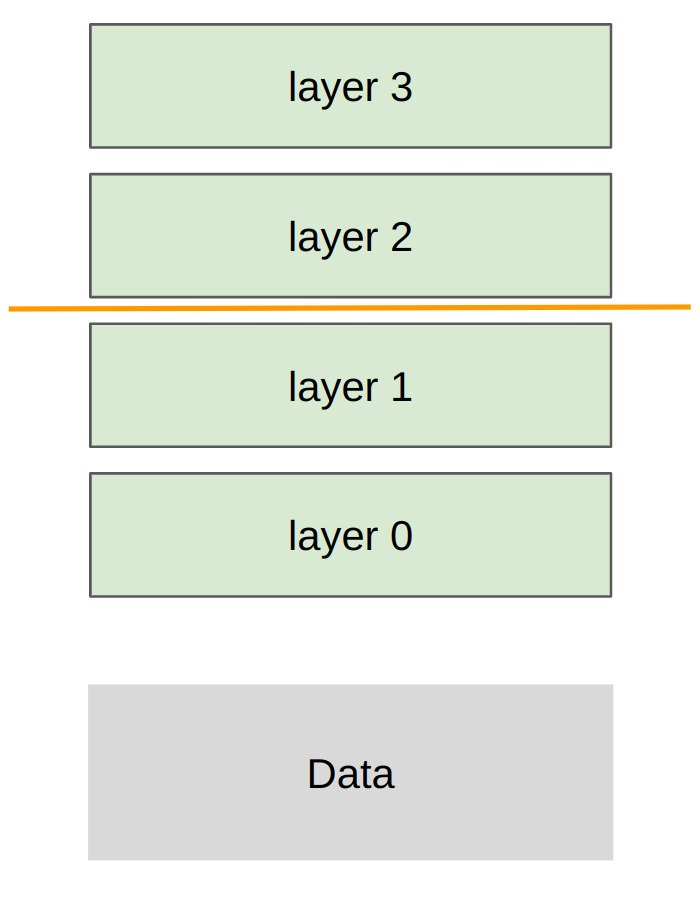
Pipeline parallelism 的 sharding strategy：

each rank gets subset of layers, transfer all data/activations

它把模型按层切开：

rank 0: layers 0,1
rank 1: layers 2,3

每个 rank 只保存自己的 layers。rank 之间传递 activations。

1.9.1 切分 layers

local_num_layers = int_divide(num_layers, world_size)

local_params = [
    get_init_params(num_dim, num_dim, rank)
    for layer in range(local_num_layers)
]

如果 num_layers=4，world_size=2，则每个 rank 持有 2 层。

1.9.2 Micro-batches

Pipeline parallelism（流水线并行） 需要 micro-batches 来减少 pipeline bubble。

micro_batch_size = int_divide(batch_size, num_micro_batches)
if rank == 0:
    micro_batches = data.chunk(chunks=num_micro_batches, dim=0)
else:
    micro_batches = [
        torch.empty(micro_batch_size, num_dim, device=cuda_if_available(rank))
        for _ in range(num_micro_batches)
    ]

如果整个 batch 一次性通过 pipeline：

rank 0 工作 -> rank 1 工作

rank 1 在 rank 0 完成前空闲，rank 0 在把数据交给 rank 1 后也可能空闲。micro-batch 的作用是把大 batch 切小，让不同 stages 同时处理不同 micro-batches。

令 pipeline stages 数为 $S$，micro-batches 数为 $M$。只考虑简单 forward pipeline，启动和排空会产生 bubble。一个直观效率近似是：

$$ \text{utilization} \approx \frac{M}{M + S - 1} $$

因此 M 越大，bubble 占比越小。但 micro-batch 太小也会降低单次 matmul 效率，并增加调度开销。

1.9.3 Rank 间 send/recv

for x in micro_batches:
    if rank - 1 >= 0:
        dist.recv(tensor=x, src=rank - 1)

    for param in local_params:
        x = x @ param
        x = F.gelu(x)

    if rank + 1 < world_size:
        dist.send(tensor=x, dst=rank + 1)

每个 rank 做三件事：

如果不是第一个 stage，从前一个 rank 接收 activation。
计算自己负责的 layers。
如果不是最后一个 stage，把 activation 发给下一个 rank。

这和 collective operations 不同：pipeline 示例用的是 point-to-point send / recv。原因是 pipeline 通信结构天然是相邻 stage 之间传 activations，不需要所有 ranks 同时参与同一个 collective。